Statistics¶

Scalar summary statistics computed over a light curve: moments, autocorrelation, variability indicators, and uncertainty rescaling.

`rms` — Root mean square¶

Syntax

cmd.rms(maskpoints=None)

Description

Compute the RMS of the light curve. The output includes the unweighted RMS, the mean magnitude, the expected RMS derived from the formal photometric uncertainties, and the number of points used. The light curve passed to subsequent commands is unchanged.

CLI equivalent: -rms.

Parameters

Parameter	Type	Description
`maskpoints`	`str` or `None`	Name of a mask variable; only points with `maskvar > 0` are included in the calculation.

Output

Suffix N is the 0-indexed pipeline command position:

Column	Description
`Mean_Mag_N`	Arithmetic mean magnitude.
`RMS_N`	Unweighted RMS.
`Expected_RMS_N`	RMS predicted from the formal photometric uncertainties (assuming they are accurate).
`Npoints_N`	Number of points used.

Examples

# Single light curve
lc = vt.LightCurve.from_file("EXAMPLES/2")
result = vt.Pipeline().rms().run(lc)
print(result.vars["Mean_Mag_0"])
print(result.vars["RMS_0"])

# Batch: compute RMS for all 10 example light curves
lcs = [vt.LightCurve.from_file(f"EXAMPLES/{i}") for i in range(1, 11)]
batch = vt.Pipeline().rms().run_batch(lcs)
print(batch.vars[["Name", "Mean_Mag_0", "RMS_0", "Expected_RMS_0"]])

`rmsbin` — Binned RMS¶

Syntax

cmd.rmsbin(nbin, bintimes, maskpoints=None)

Description

Apply a moving-mean filter to the light curve at one or more timescales and report the RMS of each filtered series. Used to characterise correlated (red) noise: as the filter window grows, white noise averages down as 1/sqrt(N) while red noise persists. The light curve passed to subsequent commands is unchanged.

bintimes are interpreted as half-widths in minutes (matching the CLI). The full filter window for each entry is 2 · bintime.

CLI equivalent: -rmsbin.

Parameters

Parameter	Type	Description
`nbin`	`int`	Number of timescale bins (filters) to apply.
`bintimes`	list of `float`	Filter half-widths in minutes; one entry per filter. Must have length `nbin`.
`maskpoints`	`str` or `None`	Name of a mask variable; only points with `maskvar > 0` are included.

Output

For each binning timescale T_i (in minutes) and command index N, vartools emits an RMSBin_<T_i>_N column (and an associated Expected_RMS_Bin_<T_i>_N column). The timescale tag in the column name is built from the input minutes value with a one-decimal-place form (e.g. 5.0 minutes becomes RMSBin_5.0_0); two distinct input values that round to the same tag will produce duplicate column names, so choose well-separated values.

Examples

lcs = [vt.LightCurve.from_file(f"EXAMPLES/{i}") for i in range(1, 11)]

# Compute binned RMS at a range of timescales, in minutes.
# (vartools truncates bin times when forming column names,
# so pick values that are well separated.)
bintimes_min = [5.0, 10.0, 60.0, 1440.0, 14400.0]
batch = vt.Pipeline().rmsbin(5, bintimes_min).run_batch(lcs)
print(batch.vars)

`chi2` — Chi-squared statistic¶

Syntax

cmd.chi2(maskpoints=None)

Description

Compute χ²/dof for the light curve relative to the error-weighted mean magnitude. A value much greater than 1 indicates the formal photometric uncertainties under-predict the observed scatter, signalling either real variability or under-estimated errors. The light curve passed to subsequent commands is unchanged.

CLI equivalent: -chi2.

Parameters

Parameter	Type	Description
`maskpoints`	`str` or `None`	Name of a mask variable; only points with `maskvar > 0` are included.

Output

Suffix N is the 0-indexed pipeline command position:

Column	Description
`Chi2_N`	χ²/dof of the light curve relative to its error-weighted mean.
`Weighted_Mean_Mag_N`	Error-weighted mean magnitude.

Examples

# Batch: chi-squared for all example light curves
lcs = [vt.LightCurve.from_file(f"EXAMPLES/{i}") for i in range(1, 11)]
batch = vt.Pipeline().chi2().run_batch(lcs)
print(batch.vars[["Name", "Chi2_0", "Weighted_Mean_Mag_0"]])

`chi2bin` — Binned chi-squared¶

Syntax

cmd.chi2bin(nbin, bintimes, maskpoints=None)

Description

Same idea as rmsbin but reports χ²/dof rather than RMS at each binning timescale. With pure white noise, the binned uncertainties shrink as 1/sqrt(N) and the binned χ² stays near 1; rising χ² with bin size signals red noise.

bintimes are half-widths in minutes. The light curve passed to subsequent commands is unchanged.

CLI equivalent: -chi2bin.

Parameters

Parameter	Type	Description
`nbin`	`int`	Number of filters.
`bintimes`	list of `float`	Filter half-widths in minutes; one entry per filter.
`maskpoints`	`str` or `None`	Name of a mask variable; only points with `maskvar > 0` are included.

Output

For each binning timescale T_i (in minutes) and command index N, vartools emits a Chi2Bin_<T_i>_N column and a Weight_Mean_Mag_Bin_<T_i>_N column. The timescale tag is formatted the same way as for rmsbin (e.g. 60.0 minutes becomes Chi2Bin_60.0_0); choose well-separated bin times to avoid duplicate column names.

Examples

lcs = [vt.LightCurve.from_file(f"EXAMPLES/{i}") for i in range(1, 11)]
bintimes_min = [5.0, 10.0, 60.0, 1440.0, 14400.0]
batch = vt.Pipeline().chi2bin(5, bintimes_min).run_batch(lcs)
print(batch.vars)

`stats` — Generic statistics¶

Syntax

cmd.stats(variables, statistics, maskpoints=None)

Description

Compute one or more general statistics on one or more light-curve vectors (e.g. t, mag, err, or any user-defined variable). Every requested statistic is computed for every listed variable, producing a STATS_<var>_<STAT>_N column for each combination. Useful for downstream variable references (e.g. computing tspan = STATS_t_MAX_0 - STATS_t_MIN_0).

variables and statistics may each be either a comma-separated string or a Python list of strings. Available statistics include mean, weightedmean, median, wmedian, stddev, meddev, medmeddev, MAD, kurtosis, skewness, pct<f> / wpct<f> (any percentile from 0 to 100), max, min, and sum.

CLI equivalent: -stats.

Parameters

Parameter	Type	Description
`variables`	`str` or list of `str`	Variable name(s) to compute statistics on. List form is joined with commas before being passed to the CLI.
`statistics`	`str` or list of `str`	Statistic name(s); see the table below. List form is joined with commas.
`maskpoints`	`str` or `None`	Name of a mask variable; only points with `maskvar > 0` contribute.

Available statistics

String	Description
`mean`	Arithmetic mean.
`weightedmean`	Mean weighted by `1/σ²`.
`median`	Median.
`wmedian`	Median weighted by light-curve uncertainties.
`stddev`	Standard deviation about the mean.
`meddev`	Standard deviation about the median.
`medmeddev`	Median absolute deviation from the median.
`MAD`	`1.483 × medmeddev` (matches stddev for a Gaussian distribution at large `N`).
`kurtosis`, `skewness`	Higher moments.
`pct<f>`	The `<f>`-th percentile (`0 < f < 100`), e.g. `pct25`.
`wpct<f>`	Weighted percentile using the light-curve uncertainties.
`max`, `min`	Maximum (`pct100`) and minimum (`pct0`).
`sum`	Sum of the elements.

Output

Per variable V, statistic S, and command index N:

Column	Description
`STATS_V_S_N`	Value of statistic `S` computed on variable `V`. The statistic name is upper-cased in the column (e.g. `STATS_mag_MEAN_0`, `STATS_t_MAX_0`).

Examples

lc = vt.LightCurve.from_file("EXAMPLES/3")

# Compute percentile and distribution statistics after adding Gaussian noise
pipe = (vt.Pipeline()
        .expr("mag2=mag+0.01*gauss()")
        .stats(
            ["mag", "mag2"],
            ["mean", "weightedmean", "median", "stddev", "MAD",
             "kurtosis", "skewness", "pct10", "pct90", "max", "min"],
        ))
result = pipe.run(lc)
print(result.vars["STATS_mag_MEAN_1"])
print(result.vars["STATS_mag_MEDIAN_1"])
print(result.vars["STATS_mag2_STDDEV_1"])

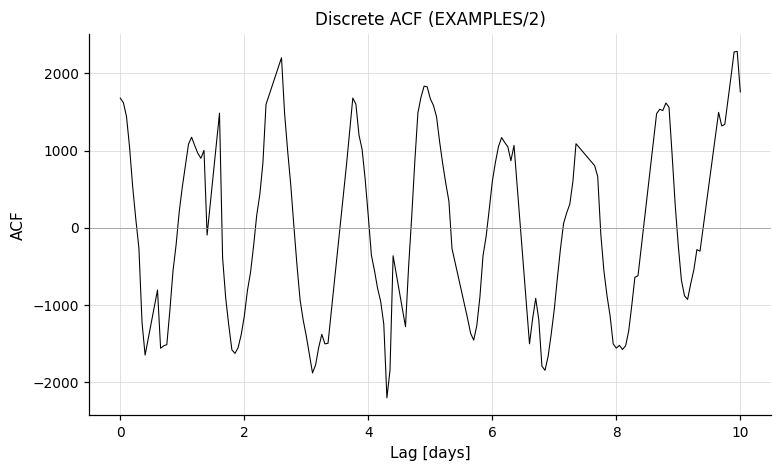
`autocorrelation` — Autocorrelation function¶

Syntax

cmd.autocorrelation(start, stop, step, save_result=True, maskpoints=None)

Description

Compute the discrete autocorrelation function (DACF) of the magnitude series following Edelson and Krolik (1988). The DACF is sampled at lags from start to stop in steps of step (all in days). Unlike the original Edelson and Krolik formulation, the formal measurement uncertainties are used in the denominator rather than the variance, which avoids imaginary values when errors are over-estimated; precede with -changeerror (in the same Pipeline) to recover the variance-based form.

The autocorrelation output file is always written to disk; save_result=False only suppresses Python capture. The file in that case is written to a temporary directory and discarded after the run.

CLI equivalent: -autocorrelation.

Parameters

Parameter	Type	Description
`start`, `stop`, `step`	`float`, `str`, numpy array, `PerLC`, or `pd.Series`	Lag range and step size (days).
`save_result`	`bool`, `str`, or `Output`	Auxiliary file output. `True` (default) captures as `result.files["autocorrelation_result_N"]`; a path string writes to that directory without capturing; `Output(path, capture=True)` does both. See Auxiliary output files and the note below.
`maskpoints`	`str` or `None`	Name of a mask variable; only points with `maskvar > 0` are included.

File is always written

The autocorrelation output file is always written to disk — autocorrelation has no option to suppress the write. Setting save_result=False only suppresses Python capture; the file is still written to a temp directory and discarded after the run completes.

Output

The command emits no per-LC scalar columns; the autocorrelation function is delivered through the auxiliary output file:

File key	Description
`result.files["autocorrelation_result_N"]`	DataFrame: time-lag (days) vs. autocorrelation. In a batch run this becomes a list of DataFrames, one per light curve.

References

Edelson, R.A. & Krolik, J.H. 1988, ApJ, 333, 646.

Examples

lc = vt.LightCurve.from_file("EXAMPLES/2")

# Default (save_result=True): ACF captured into result.files
result = vt.Pipeline().autocorrelation(0.0, 10.0, 0.05).run(lc)
acf = result.files["autocorrelation_result_0"]   # pd.DataFrame: time-lag vs autocorrelation

# save_result=False: file written to temp dir but not captured
result = vt.Pipeline().autocorrelation(0.0, 10.0, 0.05, save_result=False).run(lc)
# result.files has no "autocorrelation_result_0"

# Write to a specific directory and capture (Mode 2)
from pyvartools import Output
result = (vt.Pipeline()
        .autocorrelation(0.0, 10.0, 0.05,
                        save_result=Output("EXAMPLES/OUTDIR1", capture=True))).run(lc)
acf = result.files["autocorrelation_result_0"]   # from EXAMPLES/OUTDIR1/

# Batch — result.files["autocorrelation_result_0"] is a list of DataFrames
lcs = [vt.LightCurve.from_file(f"EXAMPLES/{i}") for i in range(1, 4)]
batch = vt.Pipeline().autocorrelation(0.0, 10.0, 0.05).run_batch(lcs)
acfs = batch.files["autocorrelation_result_0"]   # list of DataFrames, one per LC

Discrete autocorrelation function for EXAMPLES/2

`Jstet` — Stetson J-statistic¶

Syntax

cmd.Jstet(timescale, dates=None, skipnormalize=False, maskpoints=None)

Exactly one of dates= or skipnormalize=True must be given.

Description

Compute Stetson's J variability index, the L statistic, and the kurtosis of the residuals. J measures time-correlated variability by pairing observations that fall within timescale of each other (in the same time units as the light curve's time column); pairs with consistent sign of the residual contribute positively, opposite-sign pairs negatively. The second argument selects how the reported J / L are normalised:

dates="path/to/dates_file" (legacy / survey-wide mode) — the file lists JDs of every possible observation in the survey; vartools computes weight_max once from that schedule and the reported J equals J_stetson * (sum_w / weight_max). This multiplier downweights LCs missing observations relative to the full schedule. Useful for cross-LC comparison within a single survey; misleading when LCs come from different surveys / cadences.
skipnormalize=True — skip the (sum_w / weight_max) rescaling entirely and report Stetson's original J and L. Use this when comparing across surveys, or when you want the textbook definition.

CLI equivalent: -Jstet.

Parameters

Parameter	Type	Description
`timescale`	`float`	Time in the LC's time units that distinguishes "near" (correlated) from "far" (uncorrelated) observation pairs.
`dates`	`str` or `None`	Path to a survey-wide dates file (see Description). Mutually exclusive with `skipnormalize`.
`skipnormalize`	`bool`	If `True`, skip the survey-completeness rescaling and report Stetson's original J / L. Mutually exclusive with `dates`.
`maskpoints`	`str` or `None`	Name of a mask variable; only points with `maskvar > 0` are included.

Output

Suffix N is the 0-indexed pipeline command position:

Column	Description
`Jstet_N`	Stetson's J variability index (rescaled when `dates` is used; original Stetson J when `skipnormalize=True`).
`Kurtosis_N`	Kurtosis of the residuals from the mean.
`Lstet_N`	Stetson's L statistic = `J × Kurtosis` (rescaled or original, matching J).

References

Stetson, P.B. 1996, PASP, 108, 851.

Examples

# Survey-wide mode -- uses a dates file to compute the cross-LC weight_max.
lcs = [vt.LightCurve.from_file(f"EXAMPLES/{i}") for i in range(1, 11)]
batch = vt.Pipeline().Jstet(0.5, dates="EXAMPLES/dates_tfa").run_batch(lcs)
print(batch.vars[["Name", "Jstet_0", "Kurtosis_0", "Lstet_0"]])

# Textbook mode -- Stetson's original J / L, no dates file needed.
batch2 = vt.Pipeline().Jstet(0.5, skipnormalize=True).run_batch(lcs)
print(batch2.vars[["Name", "Jstet_0", "Kurtosis_0", "Lstet_0"]])

`alarm` — Alarm statistic¶

Syntax

cmd.alarm(maskpoints=None)

Description

Compute the alarm variability statistic of Tamuz, Mazeh and North (2006). The alarm is a detection statistic for coherent signals: long runs of consecutive positive or negative residuals from the mean are penalised more heavily than randomly distributed deviations of the same RMS, making it sensitive to time-correlated structure that low-order moments may miss.

CLI equivalent: -alarm.

Parameters

Parameter	Type	Description
`maskpoints`	`str` or `None`	Name of a mask variable; only points with `maskvar > 0` contribute.

Output

Suffix N is the 0-indexed pipeline command position:

Column	Description
`Alarm_N`	The alarm statistic.

References

Tamuz, O., Mazeh, T. and North, P. 2006, MNRAS, 367, 1521.

Examples

lc = vt.LightCurve.from_file("EXAMPLES/2")
result = lc.alarm()
print(result.vars["Alarm_0"])

`vonNeumann` — von Neumann ratio¶

Syntax

cmd.vonNeumann(weighted=False, maskpoints=None)

Description

Compute the von Neumann (1941) ratio η = δ² / s², where δ² = (1/(N−1)) · Σᵢ (yᵢ₊₁ − yᵢ)² is the mean-square successive difference and s² = (1/N) · Σᵢ (yᵢ − ȳ)² is the variance. For uncorrelated Gaussian noise E[η] = 2 (variance ≈ 4/N); smoothly varying (positively correlated) signals drive η well below 2; anti-correlated (alternating) signals push η above 2. Useful as a variability indicator for sparse and unevenly sampled photometric time series.

The light curve is time-sorted automatically before the calculation.

CLI equivalent: -vonNeumann.

Parameters

Parameter	Type	Description
`weighted`	`bool`	If `True`, use inverse-variance weighting: per-point weights `wᵢ = 1/σᵢ²` enter the variance and pairwise weights `w_pair_i = 1/(σᵢ² + σᵢ₊₁²)` enter the mean-square successive difference. The weighted ratio is `η_w = (2N/(N−1)) · Σ w_pair_i (yᵢ₊₁ − yᵢ)² / Σ wᵢ (yᵢ − ȳ_w)²`; the `2N/(N−1)` prefactor restores `E[η_w] = 2` for white noise regardless of the σ distribution. For homoscedastic σ the weighted form reduces exactly to the unweighted form. Points with NaN / non-positive uncertainty are dropped.
`maskpoints`	`str` or `None`	Name of a mask variable; only points with `maskvar > 0` contribute.

Output

Suffix N is the 0-indexed pipeline command position:

Column	Description
`VonNeumann_Ratio_N`	The von Neumann ratio η.

References

von Neumann, J. 1941, Annals of Mathematical Statistics, 12, 367. For astronomical applications see Sokolovsky, K. V., et al. 2017, MNRAS, 464, 274.

Examples

lc = vt.LightCurve.from_file("EXAMPLES/2")
# Unweighted: eta near 0.026 (much less than 2) reflects strong correlation.
result = lc.vonNeumann()
print(round(result.vars["VonNeumann_Ratio_0"], 5))

# Weighted variant.
result = lc.vonNeumann(weighted=True)
print(round(result.vars["VonNeumann_Ratio_0"], 5))

`percentileratios` — Robust scatter ratios¶

Syntax

cmd.percentileratios(percentilepairs=None, maskpoints=None)

Description

Compute robust scatter statistics from the magnitude distribution. For each pair of percentiles (p, q) with 0 < p < q < 100, the command emits two statistics per light curve:

amp_p_q  = pct(q) - pct(p)
asym_p_q = (pct(q) - median) / (median - pct(p))

plus one additional statistic that does not depend on the pair list:

medmeddev_over_stddev = median(|x - median(x)|) / stddev(x)

For any symmetric distribution asym → 1.0; positively-skewed distributions (heavy upper tail) produce asym > 1 and negatively-skewed distributions produce asym < 1. For independent Gaussian noise medmeddev/stddev → 0.6745 in the large-N limit.

Percentile interpolation matches the stats command, so values are directly comparable to the corresponding pct(p) columns from stats. NaN magnitudes are dropped before any statistic is computed; light curves with fewer than two finite magnitudes, and ratios with a zero denominator, produce NaN outputs.

CLI equivalent: -percentileratios.

Parameters

Parameter	Type	Description
`percentilepairs`	sequence of `(p, q)` pairs, or `None`	Percentile pairs to use. Defaults to `[(5, 95), (1, 99)]` when `None`. Each pair must satisfy `0 < p, q < 100` and `p != q`; pairs with `p > q` are silently canonicalized to `p < q`; duplicate pairs (after canonicalization) are rejected. Floating-point percentiles are accepted (e.g. `(2.5, 97.5)`).
`maskpoints`	`str` or `None`	Name of a light-curve vector; only points with `maskvar > 0` are included. The median, stddev, MAD, and all percentile statistics are computed only over the masked-in subset.

Output

Suffix N is the 0-indexed pipeline command position. The p and q values are formatted with two decimal places in the column names (e.g. PCT5.00, PCT97.50):

Column	Description
`PERCENTILERATIOS_amp_PCTp_PCTq_N`	`pct(q) - pct(p)` for pair `(p, q)`.
`PERCENTILERATIOS_asym_PCTp_PCTq_N`	`(pct(q) - median) / (median - pct(p))` for pair `(p, q)`.
`PERCENTILERATIOS_medmeddev_over_stddev_N`	`median(\|x - median(x)\|) / stddev(x)`.

Examples

lc = vt.LightCurve.from_file("EXAMPLES/2")

# Defaults (5:95 and 1:99 pairs).
result = lc.percentileratios()
print(round(result.vars["PERCENTILERATIOS_asym_PCT5.00_PCT95.00_0"], 4))

# Custom pairs incl. floating-point percentile; 95:5 auto-swaps to 5:95.
result = lc.percentileratios(percentilepairs=[(10, 90), (2.5, 97.5), (95, 5)])
print(round(result.vars["PERCENTILERATIOS_amp_PCT10.00_PCT90.00_0"], 4))
print(round(result.vars["PERCENTILERATIOS_amp_PCT2.50_PCT97.50_0"], 4))
print(round(result.vars["PERCENTILERATIOS_amp_PCT5.00_PCT95.00_0"], 4))

`beyondNsigma` — Fraction beyond N sigma¶

Syntax

cmd.beyondNsigma(Nvalues=None, useMAD=False, maskpoints=None)

Description

For each light curve and each N in Nvalues, emit two fractions:

frac_above_N = #{ x : x > median + N*sigma } / N_rej
frac_below_N = #{ x : x < median - N*sigma } / N_rej

where N_rej is the number of finite magnitudes after NaN rejection. Comparisons are strict (> and <).

By default sigma is the sample standard deviation. When useMAD=True, sigma is taken to be 1.483 * median(|x - median(x)|) instead — the Gaussian-consistent calibration of the MAD. The MAD-based scale is robust to heavy tails or outliers: outliers inflate the stddev and widen the threshold, masking themselves; using MAD recovers a tighter threshold that correctly flags the outliers.

The N=1 instance corresponds to the Beyond1Std feature of Nun et al. 2015 (the FATS package), generalized here to an arbitrary list of N values and to a choice of stddev or MAD scale.

NaN magnitudes are dropped; LCs with fewer than two finite magnitudes produce NaN outputs. When sigma == 0, the fractions are reported as zero.

CLI equivalent: -beyondNsigma.

Parameters

Parameter	Type	Description
`Nvalues`	sequence of `float`, or `None`	`N` values to evaluate. Defaults to `[1.0, 3.0, 5.0]` when `None`. Each value must be strictly positive; duplicates are rejected at construction time. Floating-point values are accepted.
`useMAD`	`bool`	If `True`, use `1.483 * MAD` instead of stddev. Default `False`.
`maskpoints`	`str` or `None`	Name of a light-curve vector; only points with `maskvar > 0` are included. The median, sigma, threshold counts, and the `N_rej` denominator are all computed over the masked-in subset.

Output

Suffix N is the 0-indexed pipeline command position; X.XX is the N value with two decimal places (e.g. N1.00, N2.50):

Column	Description
`BEYONDNSIGMA_frac_above_NX.XX_N`	Fraction of magnitudes with `x > median + N*sigma`.
`BEYONDNSIGMA_frac_below_NX.XX_N`	Fraction of magnitudes with `x < median - N*sigma`.

References

Cite Nun et al. 2015, arXiv:1506.00010 (the FATS package for variable-star feature engineering).

Examples

import numpy as np

# Defaults (N = 1, 3, 5) on a real light curve.
lc = vt.LightCurve.from_file("EXAMPLES/2")
result = lc.beyondNsigma()
print(round(result.vars["BEYONDNSIGMA_frac_above_N1.00_0"], 4))
print(round(result.vars["BEYONDNSIGMA_frac_below_N1.00_0"], 4))

# Custom float N values with the MAD-based robust scale.
result = lc.beyondNsigma(Nvalues=[0.5, 1.0, 1.5], useMAD=True)
print(round(result.vars["BEYONDNSIGMA_frac_above_N0.50_0"], 4))
print(round(result.vars["BEYONDNSIGMA_frac_above_N1.00_0"], 4))

# Synthetic Gaussian noise -> frac_above_N1 should be near 0.1587.
rng = np.random.default_rng(0)
n = 5000
gauss = vt.LightCurve.from_arrays(
    np.linspace(0, 30, n),
    rng.normal(0.0, 1.0, n),
    np.full(n, 1.0),
    name="gauss",
)
result = gauss.beyondNsigma()
above_1 = result.vars["BEYONDNSIGMA_frac_above_N1.00_0"]
print(f"frac_above_N1 = {above_1:.4f}  (Gaussian expectation: 0.1587)")

`slopestats` — Per-pair slope statistics¶

Syntax

cmd.slopestats(bintime=None, binshift=None, threshold=None,
               maxgap=None, useMAD=False, maskpoints=None)

Description

For each light curve, compute per-pair slope statistics over consecutive points after time-sorting (and optionally after binning). For pairs (t_i, m_i), (t_{i+1}, m_{i+1}), form the slope s_i = (m_{i+1} - m_i) / (t_{i+1} - t_i) and report five statistics per (LC, binsize) combination:

median_abs_dmdt = median(|s_i|)
max_abs_dmdt    = max(|s_i|)
mad_dmdt        = 1.483 * median(|s_i - median(s_i)|)
frac_above_T    = #{ s_i : s_i - <s> >  T*sigma } / N_pairs
frac_below_T    = #{ s_i : s_i - <s> < -T*sigma } / N_pairs

<s> is the mean of the slopes; deviations are mean-centered regardless of the choice of sigma flavor. Comparisons against T*sigma are strict (> and <).

By default sigma is the sample standard deviation of the slopes (normalized by N_pairs - 1). When useMAD=True, sigma is 1.483 * median(|s_i - median(s_i)|) instead (= mad_dmdt), which is more robust to heavy tails or outliers.

The bintime parameter takes a list of bin sizes in minutes (assuming the light curve time axis is in days; the kernel divides each bintime by 1440 before binning). Each binsize produces its own column set, tagged in the column name as _BTX.XX. Within each bin, an unweighted average of (t, m) is taken, and consecutive-bin slopes are formed from those averages. The binshift parameter (only valid in combination with bintime) shifts the first bin by a fraction of the binwidth: t0_bin = t[0] - binshift * binsize. Canonical use is 0 <= binshift < 1.

The maxgap parameter (in days) drops any consecutive pair whose time separation exceeds it, suppressing spurious large slopes that span long observational gaps.

The max_abs_dmdt statistic corresponds to the MaxSlope feature of Richards et al. 2011. The frac_above_T*sigma / frac_below_T*sigma statistics are slope-domain generalizations of the magnitude-domain Beyond1Std feature of the same paper, extended to a user-supplied list of T values and split into signed above/below counts.

NaN magnitudes are dropped; LCs with fewer than one surviving pair report NaN for all five stats. When sigma == 0 (all slopes equal), the threshold fractions are reported as zero while the median/max/MAD remain well-defined.

Expected values for Gaussian white noise. For magnitudes m_i ~ N(0, σ²) iid with uniform spacing dt, the slopes s_i = (m_{i+1} − m_i)/dt are Gaussian with stddev σ_s = sqrt(2)·σ/dt. Adjacent slopes have correlation −1/2 because they share a magnitude, but the median/MAD/max statistics are leading-order insensitive to that correlation. The large-N expectations are:

Statistic	Expectation
`median_abs_dmdt`	`0.6745 · σ_s ≈ 0.9540 · σ/dt`
`mad_dmdt`	`σ_s = sqrt(2) · σ/dt ≈ 1.4142 · σ/dt`
`max_abs_dmdt`	`σ_s · sqrt(2·ln N_pairs) ≈ 2·sqrt(ln N_pairs) · σ/dt` (leading order)
`frac_above_T = frac_below_T`	`1 − Φ(T)` (e.g. `0.1587` at `T=1`, `0.00135` at `T=3`, `2.87×10⁻⁷` at `T=5`)

The mad_dmdt formula is exact-in-the-limit by construction — the 1.483 factor is calibrated so that 1.483 · medmeddev(Gaussian) → σ. The max_abs_dmdt expression is the leading order of the Gumbel limit law for the maximum of N independent Gaussians (Cramér 1946, Mathematical Methods of Statistics, eq. 28.6.13); a more accurate next-order asymptotic is σ_s · ( sqrt(2·ln N_pairs) − (ln ln N_pairs + ln 4π) / (2·sqrt(2·ln N_pairs)) + γ / sqrt(2·ln N_pairs) ) with γ ≈ 0.5772 the Euler–Mascheroni constant.

These expectations assume uniform sampling. For non-uniform dt_i the slope distribution is heteroskedastic with stddev s_i = sqrt(2)·σ/dt_i; max_abs_dmdt is then dominated by the smallest dt_i rather than the typical spacing, while median_abs_dmdt and mad_dmdt remain robust and reflect a typical dt.

CLI equivalent: -slopestats.

Parameters

Parameter	Type	Description
`bintime`	sequence of `float`, or `None`	List of bin sizes in minutes. Each value must be strictly positive; duplicates are rejected at construction time. If `None`, no binning is performed.
`binshift`	`float`, or `None`	Fraction of the binwidth by which to shift the first bin. Canonical use is `0 <= binshift < 1`. Only valid when `bintime` is given.
`threshold`	sequence of `float`, or `None`	`T` values for the threshold-fraction statistics. Defaults to `[3.0]` when `None`. Each value must be strictly positive; duplicates are rejected.
`maxgap`	`float`, or `None`	Drop consecutive pairs whose time separation exceeds `maxgap` (days). Must be strictly positive.
`useMAD`	`bool`	If `True`, use `1.483 * MAD` of the slopes as `sigma`. Default `False`.
`maskpoints`	`str` or `None`	Name of a light-curve vector; only points with `maskvar > 0` are included in the calculation.

Output

Suffix N is the 0-indexed pipeline command position. Y.YY is the threshold value with two decimal places (e.g. T3.00); X.XX is the bin size in minutes with two decimal places (e.g. BT5.00, BT60.00). The _BTX.XX segment is omitted when no bintime is given.

Column	Description
`SLOPESTATS_median_abs_dmdt[_BTX.XX]_N`	Median of `\|s_i\|`.
`SLOPESTATS_max_abs_dmdt[_BTX.XX]_N`	Maximum of `\|s_i\|`.
`SLOPESTATS_mad_dmdt[_BTX.XX]_N`	`1.483 * median(\|s_i - median(s_i)\|)`.
`SLOPESTATS_frac_above_TY.YY[_BTX.XX]_N`	Fraction of slopes with `s_i - <s> > T*sigma`.
`SLOPESTATS_frac_below_TY.YY[_BTX.XX]_N`	Fraction of slopes with `s_i - <s> < -T*sigma`.

References

Cite Richards et al. 2011, ApJ, 733, 10.

Examples

import numpy as np

# Defaults (threshold T = 3, no binning) on a real light curve.
lc = vt.LightCurve.from_file("EXAMPLES/2")
result = lc.slopestats()
print(round(result.vars["SLOPESTATS_median_abs_dmdt_0"], 4))
print(round(result.vars["SLOPESTATS_max_abs_dmdt_0"], 4))

# Binning at 10 and 30 minutes with multiple thresholds and a gap filter.
result = lc.slopestats(bintime=[10, 30], threshold=[1, 3], maxgap=0.5)
print(round(result.vars["SLOPESTATS_median_abs_dmdt_BT10.00_0"], 4))
print(round(result.vars["SLOPESTATS_median_abs_dmdt_BT30.00_0"], 4))

# Synthetic white-noise slopes -> frac_above_T1 should be near 0.1587
# (Gaussian one-tailed expectation).
rng = np.random.default_rng(0)
n = 20000
gauss = vt.LightCurve.from_arrays(
    np.arange(n, dtype=float),
    rng.normal(0.0, 1.0, n),
    np.full(n, 1.0),
    name="gauss",
)
result = gauss.slopestats(threshold=[1.0, 3.0])
above_1 = result.vars["SLOPESTATS_frac_above_T1.00_0"]
print(f"frac_above_T1 = {above_1:.4f}  (Gaussian expectation: 0.1587)")

`CodyM` — Flux-asymmetry statistic M¶

Syntax

cmd.CodyM(trendwindow, outlierwindow=None, sigclip=5.0, maskpoints=None)

Description

For each light curve, compute the flux-asymmetry statistic M of Cody et al. 2014 (their Equation 7):

M = (<d_10%> - d_med) / sigma_d

where d_med is the median of the long-term-detrended, outlier-filtered light curve, sigma_d is its standard deviation, and <d_10%> is the mean of the combined faintest-decile and brightest-decile values. For magnitude-valued light curves M moves in the positive direction for dipping signatures (asymmetric toward faint excursions) and in the negative direction for bursting signatures (asymmetric toward bright excursions); a value close to zero indicates a symmetric magnitude distribution. The sign convention is reversed for flux input.

Two outlier-rejection schemes are supported:

Two-stage (paper-faithful): supply outlierwindow to build a short-timescale residual on which the sigma clip operates. Real variability is removed in that residual, so the deep dips and bright bursts M measures are not themselves clipped.
Single-stage: omit outlierwindow; the sigma clip operates directly on the trend-detrended curve. Simpler, but a deep dip or burst can clip itself and bias M toward zero.

Set sigclip=0 to disable outlier rejection entirely.

M, d_10% and dmed are reported as NaN when fewer than two points survive, when the curve is flat (sigma_d = 0), or when the two deciles would overlap; the remaining diagnostic columns stay meaningful in the flat / overlapping-decile cases.

CLI equivalent: -CodyM.

Parameters

Parameter	Type	Description
`trendwindow`	`float` or `str`	Required. Boxcar full width for the long-term detrend, in the same units as the light-curve time axis. Accepts a number, a bare variable name (vartools `var`), or an explicit `"var NAME"` / `"expr EXPR"` string for per-LC sourcing. Literal values must be `> 0`.
`outlierwindow`	`float`, `str`, or `None`	Optional. Short-timescale boxcar full width that enables the two-stage scheme. Same value forms as `trendwindow`.
`sigclip`	`float` or `str`	Outlier-rejection threshold in sigma. Default `5.0`; `0` disables rejection. Same value forms as `trendwindow`. Literal values must be `>= 0`.
`maskpoints`	`str` or `None`	Name of a light-curve vector; only points with `maskvar > 0` contribute.

Output

Column	Description
`CODYM_M_N`	The statistic `M`. NaN when the curve is flat, the deciles overlap, or fewer than two points survive.
`CODYM_d10_N`	Mean of the combined faintest-decile and brightest-decile values.
`CODYM_dmed_N`	Median of the detrended, outlier-filtered curve.
`CODYM_sigma_d_N`	Standard deviation of the detrended, outlier-filtered curve.
`CODYM_Npoints_N`	Number of points surviving the NaN/mask filter and the sigma-clip.

N is the 0-indexed command position in the pipeline.

References

Cite Cody, A. M. et al. 2014, AJ, 147, 82.

Examples

# Defaults (single-stage outlier rejection, sigclip = 5) on a real LC.
# EXAMPLES/2 contains an injected perfectly symmetric sinusoidal
# signal, so M should in principle approach zero.  In practice the
# non-uniform ground-based sampling (daily windows, weather gaps)
# biases the decile statistics and pushes M to ~0.34 here -- a
# known caveat when applying M to light curves with strong window
# functions.
result = lc.CodyM(trendwindow=10)
print(round(result.vars["CODYM_M_0"], 4))
print(int(result.vars["CODYM_Npoints_0"]))

# Sign sensitivity on real injected light curves.  EXAMPLES/3.transit
# adds a transit signal on top of the EXAMPLES/3 baseline -- M moves
# in the positive (dipping) direction.  EXAMPLES/4.microlensinject
# adds a microlensing event on top of EXAMPLES/4 -- M moves in the
# negative (bursting) direction.  trendwindow should be larger than
# the variability timescale you want to keep, so we use a longer
# window for the multi-day microlensing event than for the
# hours-long transits.
for path, tw in [("EXAMPLES/3",                  10),
                 ("EXAMPLES/3.transit",          10),
                 ("EXAMPLES/4",                 100),
                 ("EXAMPLES/4.microlensinject", 100)]:
    lc_inj = vt.LightCurve.from_file(path)
    M = lc_inj.CodyM(trendwindow=tw).vars["CODYM_M_0"]
    print(f"{path:33s}  trendwindow={tw:<4d}  M = {M:+.3f}")

`CodyQ` — Quasi-periodicity statistic Q¶

Syntax

cmd.CodyQ(period, trendwindow, phasesmooth=0.25, maskpoints=None)

Description

For each light curve, compute the quasi-periodicity statistic Q of Cody et al. 2014 (their Equation 6):

Q = (rms_resid^2 - sigma^2) / (rms_raw^2 - sigma^2)

where rms_raw is the standard deviation of the long-term-detrended light curve, rms_resid is the standard deviation of the same curve after subtraction of a boxcar-smoothed phase model at the supplied period, and sigma^2 is the mean of the per-point squared errors. Q approaches 0 for a strictly periodic light curve (the phase model captures essentially all the variance) and approaches 1 for one with no detectable periodicity (the phase model removes nothing; the denominator can collapse to a non-positive value in this regime, yielding NaN); intermediate values indicate quasi-periodic variability.

The period parameter accepts a literal number, a back-reference keyword ("ls", "aov", "pdm", "ftp", "bls", "injectharm") to the primary peak of the most-recent corresponding command in the pipeline, "fix P", "fixcolumn NAME", "list ['column' col]", a bare variable name (vartools var), or an explicit "var NAME" / "expr EXPR" string. The phase smoother is invariant under a global phase shift, so the folding epoch is fixed at the first time and is not exposed.

CLI equivalent: -CodyQ.

Parameters

Parameter	Type	Description
`period`	`float` or `str`	Required. Period (days) or one of the keyword forms above. Literal values must be `> 0`.
`trendwindow`	`float` or `str`	Required. Boxcar full width for the long-term detrend, in the same units as the light-curve time axis. Accepts a number, a bare variable name, or an explicit `"var NAME"` / `"expr EXPR"` string. Literal values must be `> 0`.
`phasesmooth`	`float` or `str`	Phase-domain boxcar full width as a fraction of the period. Default `0.25`; literal values must lie in `(0, 1]`. Accepts `var` / `expr`.
`maskpoints`	`str` or `None`	Name of a light-curve vector; only points with `maskvar > 0` contribute.

Output

Column	Description
`CODYQ_Q_N`	The statistic `Q`. NaN when `rms_raw^2 - sigma^2 <= 0` or the inputs are invalid.
`CODYQ_Period_N`	The period actually used (the resolved value for `var` / `expr` / back-reference sources).
`CODYQ_RMS_raw_N`	Standard deviation of the trend-detrended light curve.
`CODYQ_RMS_resid_N`	Standard deviation of the residual after subtracting the smoothed phase model.
`CODYQ_Sigma_N`	`sqrt(sigma^2)` = root-mean-square of the per-point errors over the surviving points.
`CODYQ_Npoints_N`	Number of points surviving the NaN / `sig <= 0` / mask filter.

N is the 0-indexed command position in the pipeline.

References

Cite Cody, A. M. et al. 2014, AJ, 147, 82.

Examples

# Literal-fix period on a real LC.
result = lc.CodyQ(period=1.234, trendwindow=10)
print(round(result.vars["CODYQ_Q_0"], 4))
print(round(result.vars["CODYQ_Period_0"], 3))

# Period sourced from a prior -aov command (back-reference).
result = vt.Pipeline([
    cmd.aov(0.5, 4.0, 0.1, 5, npeaks=1, save_periodogram=False),
    cmd.CodyQ(period="aov", trendwindow=10),
]).run(lc)
print(round(result.vars["CODYQ_Q_1"], 4))
print(round(result.vars["CODYQ_Period_1"], 4))

# Pure sinusoid evaluated at its true period -> Q ~ 0 (periodic).
rng = np.random.default_rng(0)
n = 3000
t_syn = np.arange(n, dtype=float) * 0.01
mag_syn = 0.1 * np.sin(2.0 * np.pi * t_syn / 2.0) + rng.normal(0.0, 0.01, n)
sin_lc = vt.LightCurve.from_arrays(t_syn, mag_syn, np.full(n, 0.01), name="sin")
result = sin_lc.CodyQ(period=2.0, trendwindow=100)
print(f"sinusoid Q at true P = {result.vars['CODYQ_Q_0']:.3f}  (expect ~ 0)")

`structurefunction` — Ensemble structure function¶

Syntax

cmd.structurefunction(
    bins,
    Nbins=None,
    edges=None,
    lagrange=None,
    estimator="squared",
    fitDRW=False,
    sigma0=None,
    tau0=None,
    reportsfvalsintable=None,
    save_result=False,
    maskpoints=None,
)

Description

Compute the ensemble structure function (SF) of a light curve on user-specified lag bins, and optionally fit a damped-random-walk (DRW / Ornstein–Uhlenbeck / CAR(1)) model to it.

Two estimators are supported, selected by estimator:

"squared" (default) — squared-difference form with bin-averaged noise subtraction (the D^(1)(tau) of Simonetti, Cordes & Heeschen 1985):
```
SF^2(dt) = <(m_j - m_i)^2>_pairs - <sigma_i^2 + sigma_j^2>_pairs
SF(dt)   = sqrt(SF^2)
```
Bins where the noise-subtracted variance is non-positive are NaN.
"mad" — absolute-deviation form with per-pair noise subtraction (Hughes, Aller & Aller 1992; Schmidt et al. 2010, their Equation 2):
```
V(dt) = <(sqrt(pi)/2) * |m_j - m_i| - sqrt(sigma_i^2 + sigma_j^2)>_pairs
```
More robust to outliers, biased low when the intrinsic variance approaches the photometric noise floor; bins whose averaged value goes non-positive are NaN.

Per-bin error bars are reported as sigma_SF = SF / sqrt(2 N_eff) (squared) or sigma_SF = SF / sqrt(N_eff / (pi/2 - 1)) (mad), with N_eff = min(N_pairs, N_obs/2) capping the effective number of independent pairs.

When fitDRW=True, a DRW model is fit to the well-determined SF bins. The DRW analytic SF is

SF_DRW(dt) = SF_inf * sqrt(1 - exp(-dt / tau)),    SF_inf = sqrt(2) * sigma_long

This is the MacLeod et al. 2010 parameterisation; the underlying CAR(1) model was introduced for AGN optical variability by Kelly, Bechtold & Siemiginowska 2009. The fit minimises chi^2 = sum [(SF_obs - SF_model) / sigma_SF]^2 via a downhill simplex on (log SF_inf, log tau); the reported scalar amplitude is sigma_long (mag). To convert to Kelly's SDE driving-noise amplitude sigma_K (mag · day^(-1/2)) use sigma_K = sigma_long * sqrt(2 / tau).

CLI equivalent: -structurefunction.

Parameters

Parameter	Type	Description
`bins`	`str`	Required. One of `"log"`, `"linear"`, `"edges"`.
`Nbins`	`int` or `None`	Required for `bins="log"` / `"linear"`. Must be `>= 2`.
`edges`	sequence of `float` or `None`	Required for `bins="edges"`. Strictly increasing positive bin edges; produces `len(edges) - 1` bins.
`lagrange`	tuple `(lagmin, lagmax)` or `None`	Optional. Fixes the lag range for `log` / `linear` binning. Each element accepts a number, a bare variable name (vartools `var`), or an explicit `"var NAME"` / `"expr EXPR"` string. Literals must satisfy `lagmin > 0`, `lagmax > lagmin`.
`estimator`	`"squared"` or `"mad"`	Optional. SF estimator family. Default `"squared"`.
`fitDRW`	`bool`	Optional. Fit a DRW model. Default `False`.
`sigma0`	`float` or `str` or `None`	Optional (only with `fitDRW=True`). Initial guess for `sigma_long`. Accepts `var` / `expr`. Literals must be `> 0`.
`tau0`	`float` or `str` or `None`	Optional (only with `fitDRW=True`). Initial guess for `tau`. Accepts `var` / `expr`. Literals must be `> 0`.
`reportsfvalsintable`	sequence of `float` or `None`	Optional. Strictly increasing list of positive lag values; for each, emit four scalar columns.
`save_result`	`bool`, `str`, or `Output`	Optional. Controls the `.sf` aux file (full SF curve). `False` (default): no file. `True`: write to pipeline temp dir, capture into `result.files["structurefunction_result_N"]`. Path string: write to that dir, no capture.
`maskpoints`	`str` or `None`	Optional. Mask variable; only points with `maskvar > 0` contribute.

Output

Suffix N is the 0-indexed pipeline command position.

When fitDRW=True:

Column	Description
`STRUCTUREFUNCTION_SIGMA_N`	`sigma_long`, the MacLeod 2010 long-term magnitude standard deviation. NaN on non-convergence.
`STRUCTUREFUNCTION_TAU_N`	DRW damping time-scale. NaN on non-convergence.
`STRUCTUREFUNCTION_CHI2_N`	Best-fit chi^2.
`STRUCTUREFUNCTION_DOF_N`	Well-determined-bin count minus 2.
`STRUCTUREFUNCTION_CONVERGED_N`	`1` if converged, `0` otherwise.

When reportsfvalsintable=[e1,...,en], for each e_k (k = 0..n-1):

Column	Description
`STRUCTUREFUNCTION_DT_k_N`	Actual bin centre containing `e_k`. NaN if out of range.
`STRUCTUREFUNCTION_SF_k_N`	SF value for that bin. NaN if noise-dominated or empty.
`STRUCTUREFUNCTION_SIGMA_SF_k_N`	Per-bin error bar. NaN if `SF_k` is NaN.
`STRUCTUREFUNCTION_NPAIRS_k_N`	Number of pairs in the bin. `0` if out of range.

When save_result=True, result.files["structurefunction_result_N"] holds a four-column aux file (dt_center SF sigma_SF n_pairs); bins with no pairs or noise-dominated SF appear with SF = sigma_SF = NaN.

References

Cite Simonetti, Cordes & Heeschen 1985, ApJ, 296, 46, if you use estimator="squared".

Cite Hughes, Aller & Aller 1992, ApJ, 396, 469 and Schmidt et al. 2010, ApJ, 714, 1194, if you use estimator="mad".

Cite Kelly, Bechtold & Siemiginowska 2009, ApJ, 698, 895 and MacLeod et al. 2010, ApJ, 721, 1014, if you use fitDRW.

Examples

# Structure function values at three chosen lags on EXAMPLES/2.
result = lc.structurefunction(
    bins="log", Nbins=20,
    reportsfvalsintable=[0.1, 1.0, 10.0],
)
print(f"DT_0 = {result.vars['STRUCTUREFUNCTION_DT_0_0']:.4f}")
print(f"SF_0 = {result.vars['STRUCTUREFUNCTION_SF_0_0']:.4f}")
print(f"SF_2 = {result.vars['STRUCTUREFUNCTION_SF_2_0']:.4f}")
print(f"NPAIRS_2 = {int(result.vars['STRUCTUREFUNCTION_NPAIRS_2_0'])}")

# DRW fit on the same LC.  EXAMPLES/2 is an injected sinusoid, so the
# DRW is the wrong model and chi^2 / dof is large -- this is how the
# fit flags model misspecification.  Recovered (sigma_long, tau) on
# real DRW data (e.g. quasar optical light curves with adequate
# baseline) approach the input values.
result = lc.structurefunction(bins="log", Nbins=20, fitDRW=True)
print(f"sigma_long = {result.vars['STRUCTUREFUNCTION_SIGMA_0']:.4f}")
print(f"tau        = {result.vars['STRUCTUREFUNCTION_TAU_0']:.4f}")
print(f"chi2/dof   = {result.vars['STRUCTUREFUNCTION_CHI2_0'] / result.vars['STRUCTUREFUNCTION_DOF_0']:.1f}")
print(f"converged  = {int(result.vars['STRUCTUREFUNCTION_CONVERGED_0'])}")

`drwfit` — Direct DRW maximum-likelihood fit¶

Syntax

cmd.drwfit(
    mean=None,
    mean_value=None,
    sigma0=None,
    tau0=None,
    mean0=None,
    save_result=False,
    correctlc=None,
    modelvar=None,
    maskpoints=None,
)

Description

Fit a damped-random-walk (DRW / Ornstein–Uhlenbeck / CAR(1)) model directly to a light curve by maximum likelihood, using the Kelly, Bechtold & Siemiginowska 2009 state-space recursion (their Equations 6–13). Each likelihood evaluation is O(N) with no matrix inversion, and a downhill simplex (Nelder–Mead) minimises -2 ln L over (log sigma_long, log tau) — jointly with mu when the mean is fit.

This direct-likelihood method recovers tau substantially more accurately than fitting a DRW to the structure function (structurefunction with fitDRW=True), especially on short baselines (MacLeod et al. 2010 Section 4.2; Kelly 2009 Section 3.1). The reported amplitude DRWFIT_SIGMA_N is sigma_long (the MacLeod 2010 long-term magnitude standard deviation, mag) — the same quantity structurefunction reports, so the two are directly comparable. To convert to Kelly's SDE driving-noise amplitude sigma_K (mag · day^(-1/2)) use sigma_K = sigma_long * sqrt(2 / tau).

The long-term mean is controlled by mean (vartools default "fit"): "fit" fits mu jointly; "fix" (with mean_value) holds it at a fixed value; "subtract" removes the weighted mean before fitting, in which case DRWFIT_MU_N is NaN. The two DRWFIT_DLNL_* columns are likelihood-ratio detection indicators against the pure-noise and tau -> infinity limits.

Set correctlc="smoothed" (or "forecast") to replace the in-memory light curve with the DRW residuals before passing it downstream: "smoothed" subtracts the Rauch–Tung–Striebel smoothed model (past and future points), whitening toward the noise floor; "forecast" subtracts the one-step-ahead Kalman forecast (past points only), retaining unexplained variability. Set modelvar=("smoothed", name) (or ("forecast", name)) to instead store the DRW model in a new light-curve variable without altering the curve.

CLI equivalent: -drwfit.

Parameters

Parameter	Type	Description
`mean`	`"fit"`, `"subtract"`, `"fix"`, or `None`	Optional. Long-term-mean handling. `None` (default) uses the vartools default (`"fit"`).
`mean_value`	`float` or `str` or `None`	Required for, and only valid with, `mean="fix"`. The fixed `mu`. Accepts a number, a bare variable name (`var`), or a `"var NAME"` / `"expr EXPR"` string.
`sigma0`	`float` or `str` or `None`	Optional. Simplex initial guess for `sigma_long`. Accepts `var` / `expr`. Literals must be `> 0`.
`tau0`	`float` or `str` or `None`	Optional. Simplex initial guess for `tau`. Accepts `var` / `expr`. Literals must be `> 0`.
`mean0`	`float` or `str` or `None`	Optional. Simplex initial guess for `mu` (when the mean is fit). Accepts `var` / `expr`.
`save_result`	`bool`, `str`, or `Output`	Optional. Controls the `.drwfit` aux file (eight per-point columns). `False` (default): no file. `True`: write to pipeline temp dir, capture into `result.files["drwfit_result_N"]`. Path string: write to that dir, no capture.
`correctlc`	`"smoothed"`, `"forecast"`, or `None`	Optional. Replace the in-memory light curve with the smoothed or forecast DRW residuals.
`modelvar`	`(mode, varname)` or `None`	Optional. Store the DRW model in a new variable. `mode` is `"smoothed"` or `"forecast"`.
`maskpoints`	`str` or `None`	Optional. Mask variable; only points with `maskvar > 0` contribute.

Output

Suffix N is the 0-indexed pipeline command position.

Column	Description
`DRWFIT_SIGMA_N`	`sigma_long`, the MacLeod 2010 long-term magnitude standard deviation (mag).
`DRWFIT_TAU_N`	DRW damping time-scale (time-axis units).
`DRWFIT_MU_N`	Fitted long-term mean. NaN when `mean="subtract"`.
`DRWFIT_LNL_N`	Best-fit `ln L`.
`DRWFIT_DLNL_NOISE_N`	`ln L_best - ln L` at the `sigma_long -> 0` (pure-noise) limit.
`DRWFIT_DLNL_INF_N`	`ln L_best - ln L` at the `tau -> infinity` limit.
`DRWFIT_CONVERGED_N`	`1` if the simplex converged, `0` otherwise.

When save_result=True, result.files["drwfit_result_N"] holds an eight-column per-point table (t x sig_meas x_hat_fwd Omega_fwd chi_fwd x_smoothed Omega_smoothed) from the forward Kalman filter and the RTS backward smoother, with NaN rows preserved for filtered-out points.

References

Cite Kelly, Bechtold & Siemiginowska 2009, ApJ, 698, 895 and MacLeod et al. 2010, ApJ, 721, 1014, if you use this command.

Examples

# Direct maximum-likelihood DRW fit on EXAMPLES/2.  The LC carries an
# injected sinusoid rather than genuine DRW variability, so the recovered
# parameters describe the best DRW approximation to that signal; on real
# DRW data (e.g. quasar optical light curves with adequate baseline) the
# recovered (sigma_long, tau) approach the input values.
result = lc.drwfit()
print(f"sigma_long = {result.vars['DRWFIT_SIGMA_0']:.4f}")
print(f"tau        = {result.vars['DRWFIT_TAU_0']:.4f}")
print(f"mu         = {result.vars['DRWFIT_MU_0']:.4f}")
print(f"converged  = {int(result.vars['DRWFIT_CONVERGED_0'])}")

# Subtract the smoothed DRW model in place, then check the chi^2 of the
# whitened light curve with a chained -chi2.
result = lc.drwfit(correctlc="smoothed").chi2()
chi2_key = next(k for k in result.vars.index if "Chi2" in k)
print(f"chi2/dof after correction = {result.vars[chi2_key]:.3f}")

# Store the smoothed DRW model in a new variable instead of correcting,
# then summarise it with -stats.
result = lc.drwfit(modelvar=("smoothed", "drwmod")).stats("drwmod", "mean,stddev")
mean_key = next(k for k in result.vars.index if "drwmod" in k and "MEAN" in k)
print(f"model mean = {result.vars[mean_key]:.4f}")

`runlength` — Run-length statistics about the median and MAD¶

Syntax

cmd.runlength(
    k=3.0,
    maskpoints=None,
)

Description

Characterize runs of consecutive points (in time order) relative to the median magnitude and the median absolute deviation. A run is a maximal block of consecutive points that all satisfy one condition. Let m be the median of the (NaN- and mask-filtered) magnitudes and D = MAD = 1.483 * median(|x - m|) their median absolute deviation — the same 1.483-scaled estimator reported by stats, so the band m ± k*D is roughly ±k Gaussian standard deviations. Four conditions are tracked: above (x > m), below (x < m), outhigh (x - m > k*D), and outlow (x - m < -k*D).

Comparisons are strict, so a point exactly at the median is in band and breaks both the above and below runs. The two outlier conditions are sign-specific: a band excursion that crosses from the high side to the low side ends one run and begins another (there is no combined sign-agnostic outlier run). For each condition the command reports the longest run, the number of runs, and the mean run length (npoints / nruns, NaN when there are no runs).

Long runs above or below the median flag low-frequency coherent variability or a residual trend; long outlier runs flag sustained excursions (flares, blends, systematics) as opposed to isolated bad points. This is a fast, robust serial-coherence descriptor that complements the scatter statistics (rms, chi2, the MAD of stats) and the asymmetry / quasi-periodicity statistics CodyM / CodyQ. The light curve is sorted in time before the scan if it is not already in time order.

CLI equivalent: -runlength.

Parameters

Parameter	Type	Description
`k`	`float` or `str`	Optional. Outlier band half-width in MAD units. Default `3.0`; literals must be `>= 0`. Accepts a number, a bare variable name (`var`), or a `"var NAME"` / `"expr EXPR"` string. Emitted on the command line only when it differs from the default.
`maskpoints`	`str` or `None`	Optional. Mask variable; only points with `maskvar > 0` contribute.

Output

Suffix N is the 0-indexed pipeline command position. For each of the four conditions ABOVE, BELOW, OUTHIGH, OUTLOW:

Column	Description
`RUNLENGTH_<COND>_MAXLEN_N`	Longest run satisfying the condition.
`RUNLENGTH_<COND>_NRUNS_N`	Number of runs.
`RUNLENGTH_<COND>_MEANLEN_N`	Mean run length (NaN when there are no runs).

plus RUNLENGTH_MEDIAN_N (the median m), RUNLENGTH_MAD_N (the 1.483-scaled D), and RUNLENGTH_K_N (the k used). When no point survives filtering, the run statistics are 0 / 0 / NaN and the median and MAD are NaN.

References

The count of runs about the median underlies the Wald–Wolfowitz runs test (Wald & Wolfowitz 1940, Ann. Math. Statist., 11, 147); runlength reports the descriptive run statistics themselves rather than that test statistic or its p-value. No citation is required to use this command.

Examples

# Run-length statistics about the median and the +/-k*MAD band on EXAMPLES/2.
# The injected sinusoid produces long above/below runs and, at the default
# k=3, no outlier runs (the band is wider than the sinusoid amplitude).
result = lc.runlength()
print(f"longest above-median run = {int(result.vars['RUNLENGTH_ABOVE_MAXLEN_0'])}")
print(f"longest below-median run = {int(result.vars['RUNLENGTH_BELOW_MAXLEN_0'])}")
print(f"median = {result.vars['RUNLENGTH_MEDIAN_0']:.4f}, "
      f"MAD = {result.vars['RUNLENGTH_MAD_0']:.4f}")

# Tighten the band to +/-0.5*MAD so the sinusoid peaks and troughs register
# as sustained outlier runs.  The high and low excursions are tracked
# separately (sign-specific outlier conditions).
result = lc.runlength(k=0.5)
print(f"outhigh: {int(result.vars['RUNLENGTH_OUTHIGH_NRUNS_0'])} runs, "
      f"longest {int(result.vars['RUNLENGTH_OUTHIGH_MAXLEN_0'])}")
print(f"outlow:  {int(result.vars['RUNLENGTH_OUTLOW_NRUNS_0'])} runs, "
      f"longest {int(result.vars['RUNLENGTH_OUTLOW_MAXLEN_0'])}")

Statistics¶

rms — Root mean square¶

rmsbin — Binned RMS¶

chi2 — Chi-squared statistic¶

chi2bin — Binned chi-squared¶

stats — Generic statistics¶

autocorrelation — Autocorrelation function¶

Jstet — Stetson J-statistic¶

alarm — Alarm statistic¶

vonNeumann — von Neumann ratio¶

percentileratios — Robust scatter ratios¶

beyondNsigma — Fraction beyond N sigma¶

slopestats — Per-pair slope statistics¶

CodyM — Flux-asymmetry statistic M¶

CodyQ — Quasi-periodicity statistic Q¶

structurefunction — Ensemble structure function¶

drwfit — Direct DRW maximum-likelihood fit¶

runlength — Run-length statistics about the median and MAD¶

`rms` — Root mean square¶

`rmsbin` — Binned RMS¶

`chi2` — Chi-squared statistic¶

`chi2bin` — Binned chi-squared¶

`stats` — Generic statistics¶

`autocorrelation` — Autocorrelation function¶

`Jstet` — Stetson J-statistic¶

`alarm` — Alarm statistic¶

`vonNeumann` — von Neumann ratio¶

`percentileratios` — Robust scatter ratios¶

`beyondNsigma` — Fraction beyond N sigma¶

`slopestats` — Per-pair slope statistics¶

`CodyM` — Flux-asymmetry statistic M¶

`CodyQ` — Quasi-periodicity statistic Q¶

`structurefunction` — Ensemble structure function¶

`drwfit` — Direct DRW maximum-likelihood fit¶

`runlength` — Run-length statistics about the median and MAD¶