Filtering and Detrending
Commands for removing outliers, applying smoothing filters, restricting the time range of light curves, and saving and restoring light curve states.
-clip
-clip <"var" sigclipvar | "expr" sigclipexpr | sigclip>
    <"var" itervar | "expr" iterexpr | iter>
    ["niter" <"var" nvar | "expr" nexpr | n>] ["median"]
    ["markclip" var ["noinitmark"]]
Sigma-clip the light curves. Points with errors ≤ 0 or NaN magnitude values are always removed. If sigclip ≤ 0, sigma-clipping is not performed but invalid points (err ≤ 0 or NaN magnitude) are still removed. The output table includes the number of points that were clipped.
Python equivalent: clip.
Parameters
sigclip— Clipping threshold in units of the standard deviation.iter—1for iterative clipping (continue until no further points are removed);0for a single pass."niter" n— Clip for a fixed number of iterationsn."median"— Clip with respect to the median rather than the mean."markclip" var— Instead of removing clipped points, mark them: points that survive clipping receivevar = 1; clipped points receivevar = 0. The light curve length is unchanged."noinitmark"— Use the existing values ofvaras an initial clipping mask. Only points withvar = 1are considered for further clipping.
Examples
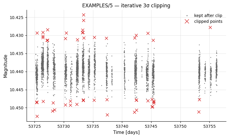
Example 1. Calculate the RMS before and after applying iterative 3-sigma clipping, then write the clipped light curve to a file.
Output:
Name           = EXAMPLES/5
Mean_Mag_0     =  10.43962
RMS_0          =   0.00288
Expected_RMS_0 =   0.00114
Npoints_0      =  3903
Nclip_1        =    51
Mean_Mag_2     =  10.43961
RMS_2          =   0.00267
Expected_RMS_2 =   0.00114
Npoints_2      =  3852
-medianfilter
Apply a running high-pass or low-pass filter to the light curve.
Python equivalent: medianfilter.
Parameters
time— Half-window width in the same units as the time coordinate. All points withintimeof a given observation contribute to the local statistic.- Default (high-pass) behavior: the local median magnitude is subtracted from each observation.
"average"— Use the running mean instead of the median."weightedaverage"— Use the running weighted mean instead of the median."replace"— Replace each point with the running statistic rather than subtracting it. This converts the command to a low-pass filter.
Examples
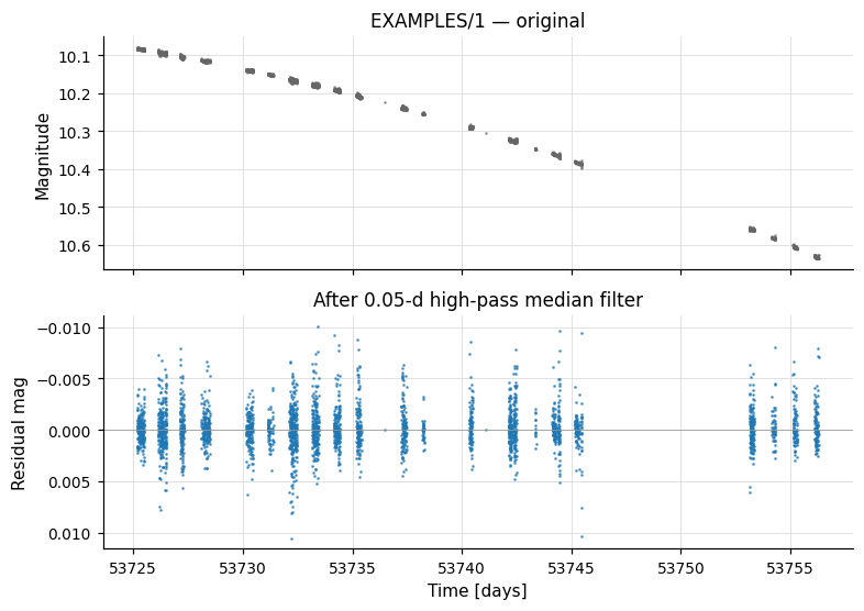
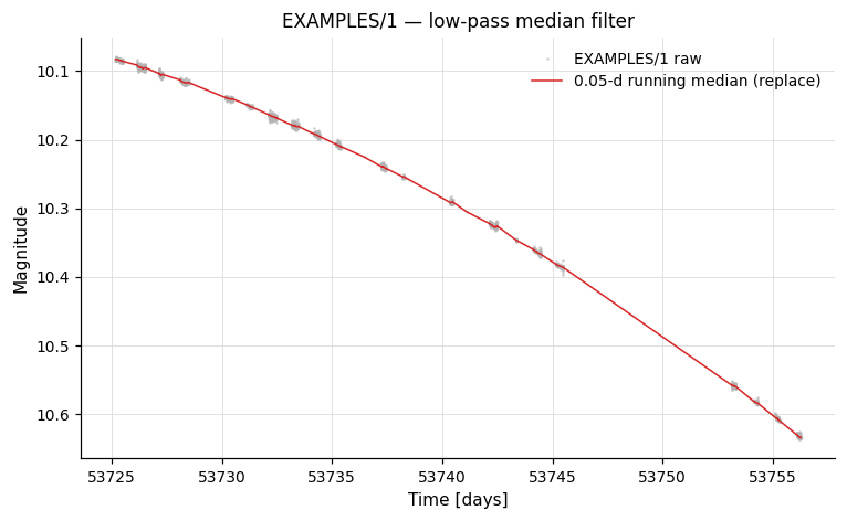
Example 1. Apply a high-pass and a low-pass median filter (0.05-day timescale) to a light curve, saving and restoring the light curve state between the two filter passes.
vartools -i EXAMPLES/1 -oneline -chi2 \
    -savelc \
    -medianfilter 0.05 \
    -chi2 -o EXAMPLES/OUTDIR1/1.medianhighpass \
    -restorelc 1 \
    -medianfilter 0.05 replace \
    -chi2 -o EXAMPLES/OUTDIR1/1.medianlowpass
Output:
Name                 = EXAMPLES/1
Chi2_0               = 34711.71793
Weighted_Mean_Mag_0  =  10.24430
Chi2_3               =   5.95454
Weighted_Mean_Mag_3  =  -0.00009
Chi2_7               = 34727.65120
Weighted_Mean_Mag_7  =  10.24440
-harmonicfilter
Syntax
-harmonicfilter <"aov" | "ls" | "both" | "injectharm"
    | "fix" Nper <"var" v | "expr" e | per1> ... <"var" v | "expr" e | perN>
    | "list" Nper ["column" col1]> Nharm Nsubharm
    omodel [model_outdir] ["fitonly"]
    ["outampphase" | "outampradphase" | "outRphi" | "outRradphi"]
    ["clip" <"var" cvar | "expr" cexpr | val>]
Description
Fit and optionally subtract a harmonic (Fourier) series from the light curve at one or more known periods, i.e. whiten the light curve against those periods. The model has the form:
sum_{i=1}^{Nper}(
    sum_{k=0}^{Nharm_i}(a_i_k·sin(2π(k+1)f_i·t) + b_i_k·cos(2π(k+1)f_i·t))
  + sum_{k=0}^{Nsubharm_i}(c_i_k·sin(2π f_i·t/(k+1)) + d_i_k·cos(2π f_i·t/(k+1)))
)
By default the whitened light curve is passed to the next command; use "fitonly" to suppress subtraction. Use -fourierfilter instead when you want a full-band high/low/band-pass filter without specifying periods in advance.
-Killharm is accepted as a synonym for backward compatibility — same syntax and behaviour, but the output-column prefix is Killharm_* and the model-file suffix is .killharm.model instead of .harmonicfilter.model.
Python equivalent: harmonicfilter.
Parameters
| Parameter | Description |
|---|---|
"aov" |
Period from the most recent -aov or -aov_harm command. |
"ls" |
Period from the most recent -LS command. |
"both" |
Two periods: one from -aov, one from -LS. |
"injectharm" |
Period from the most recent -Injectharm command. |
"fix" Nper per1 ... perN |
Nper fixed periods given on the command line. |
"list" Nper ["column" col1] |
Nper periods read from the input-list file. |
Nharm |
Higher harmonics included (frequencies 2f₀, 3f₀, … (Nharm+1)f₀). |
Nsubharm |
Sub-harmonics included (frequencies f₀/2, f₀/3, … f₀/(Nsubharm+1)). |
omodel [outdir] |
1 to write the model LC (suffix .harmonicfilter.model); 0 to skip. |
"fitonly" |
Compute the model but do not subtract it from the LC. |
"outampphase" |
Output amplitudes A_k = sqrt(a_k² + b_k²) and phases φ_k = atan2(-b_k, a_k)/(2π) instead of raw coefficients. |
"outampradphase" |
Same as "outampphase" but phases in radians. |
"outRphi" |
Output relative amplitudes R_k1 = A_k/A_1 and phases φ_k1 = φ_k − k φ_1 in units of 0 to 1. |
"outRradphi" |
Same as "outRphi" but phases in radians. |
"clip" val |
Fit the model, clip residuals at val σ, then refit to the surviving points. |
Output columns: HarmonicFilter_Mean_Mag_N, HarmonicFilter_Period_k_N, plus per-period harmonic coefficients in one of four representations ({Sin,Cos}coeff, {Amplitude,Phase}, R/Phi, etc.) selected by the outampphase / outRphi family.
Examples
Example 1. Search for a periodic signal in EXAMPLES/2 with Lomb-Scargle, then fit and subtract a sinusoid at the LS period using -harmonicfilter. The two -rms and -chi2 calls show how the statistics change after subtraction. Only the fundamental is fit (no harmonics or sub-harmonics), and the model is not written to disk.
vartools -i EXAMPLES/2 -oneline \
    -LS 0.1 10. 0.1 1 0 \
    -rms -chi2 \
    -harmonicfilter ls 0 0 0 \
    -rms -chi2
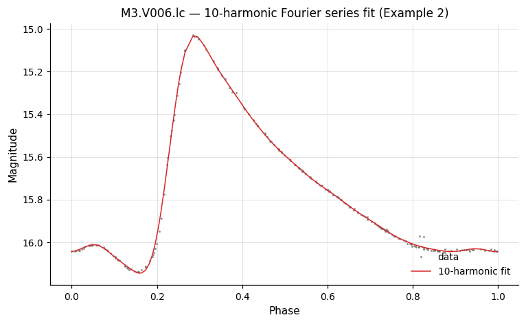
Example 2. Fit a 10-harmonic Fourier model to the RR Lyrae light curve EXAMPLES/M3.V006.lc at a fixed period of 0.514333 days. The model is written to EXAMPLES/OUTDIR1/M3.V006.lc.harmonicfilter.model, the LC is left unchanged (fitonly), and amplitudes/phases are reported in the relative R_k1, φ_k1 form (outRphi) — that representation can be fed directly to -Injectharm to inject a signal with the same RR-Lyrae shape but a different overall amplitude or phase.
vartools -i EXAMPLES/M3.V006.lc -oneline \
    -harmonicfilter fix 1 0.514333 10 0 1 \
        EXAMPLES/OUTDIR1/ fitonly outRphi
-Killharm
Backward-compatible synonym for -harmonicfilter —
same syntax, same behaviour. Output columns produced by the legacy name
are prefixed with Killharm_* instead of HarmonicFilter_*, and the
model-file suffix is .killharm.model instead of .harmonicfilter.model,
so existing scripts that read these columns or files keep working.
New code should use -harmonicfilter.
-fourierfilter
-fourierfilter
    <"full" |
     "highpass" "minfreq" <"var" v | "expr" e | "fix" val | "fixcolumn" <col> | "list" ["column" col]> |
     "lowpass"  "maxfreq" <...> |
     "bandpass" "minfreq" <...> "maxfreq" <...> |
     "bandcut"  "minfreq" <...> "maxfreq" <...>>
    ["filterexpr" expr ["freqvar" name]]
    ["fullspec"] ["forcefft"]
    ["taper" <"linear"|"cosine"|"blackman"|"kaiser"> "deltafreq" val ["beta" val]]
    ["resample" <"delmin"|"fix" v|"var" n|"expr" e>
        ["gapbreak" <"fix" v|"expr" e|"frac_min_sep" v|"frac_med_sep" v|"percentile_sep" v>]]
    ["padmode" <"wrap"|"reflect"|"zero"> ["padfrac" val]]
    ["ofourier" outdir ["nameformat" fmt]]
    ["nowarn"]
Apply a Fourier-domain filter to the whole light curve. A band filter
and/or an analytic filterexpr is applied in frequency space, and the
filtered light curve replaces the input (except in a subtract-mode
special case below). The command uses GSL's mixed-radix complex FFT
(gsl_fft_complex_forward / gsl_fft_complex_inverse), so a GSL-enabled
build is required. This is distinct from
-harmonicfilter, which fits a Fourier series at
one or more known periods.
There are two algorithmic paths:
-
Uniform sampling (or
forcefft) — the FFT runs directly on the input samples. Before the FFT the weighted mean is subtracted and the signal is optionally edge-padded (seepadmode). The mask is applied to each complex bin in frequency space, the IFFT returns the filtered signal, padding is discarded, and the mean is added back. The FFT bin spacing isdf_fft = 1/(Ntot·delmin), whereNtot = Nfor the defaultpadmode="wrap"orNtot = N + 2·floor(padfrac·N)forreflect/zeropadding. -
resample <delta>— the light curve is linearly interpolated onto a uniform grid at spacing<delta>first. Path 1 is then run on that uniform grid, and the filtered result is linearly interpolated back to the original sample times. Required for non-uniformly- sampled data. Can be combined withgapbreakto split the light curve at large gaps and filter each segment independently.
Non-uniform sampling without resample
If the detected sampling is non-uniform and resample is not given
(and forcefft is not given), the command prints a warning to
stderr and skips the filter for that light curve — the mag
column is passed through unchanged to the next command. The
command does not abort the pipeline; subsequent LCs and
subsequent pipeline commands process normally. The output columns
for the skipped LC are set to:
FourierFilter_Mean_Mag_N = 0FourierFilter_RMS_In_N = <input LC RMS>(computed before the skip)FourierFilter_RMS_Out_N = FourierFilter_RMS_In_N(signals no filter was applied)FourierFilter_Nfreqcalc_N = 0FourierFilter_Nfreqfilt_N = 0
The warning can be silenced with nowarn.
Subtract vs. replace (path 1 only)
In path 1, modes highpass and bandcut without filterexpr or
fullspec compute the reject-band reconstruction and subtract
it from the input light curve — preserving the original pass-band
content exactly (modulo FFT round-off) at the original sample
times. All other path-1 cases, and path 2 always, replace the
light curve with the pass-band reconstruction.
Filter modes
| Mode | Keeps | Rejects |
|---|---|---|
"full" |
Everything (use with "filterexpr" for an analytic filter). |
— |
"highpass" |
f ≥ minfreq |
f < minfreq |
"lowpass" |
f ≤ maxfreq |
f > maxfreq |
"bandpass" |
minfreq ≤ f ≤ maxfreq |
outside |
"bandcut" |
outside [minfreq, maxfreq] |
inside |
Each of minfreq / maxfreq accepts the standard fix, list, fixcolumn, expr, or var forms.
Analytic filter — "filterexpr"
"filterexpr" expr ["freqvar" name] applies an analytic filter W(f)
on top of the selected band. The expression is evaluated at each
trial frequency and the cos/sin coefficients at that frequency are
multiplied by the result. The frequency variable is named f by
default (e.g. "filterexpr 'exp(-(f/0.5)^2)'") and can be renamed
with "freqvar name" to avoid collisions with user variables. The
expression may reference constants and per-star scalars but not
light-curve vectors.
Edge tapering — "taper"
By default the filter cuts are brick walls. "taper" softens each
cut edge with a smooth transition of half-width deltafreq centered
on the edge, reducing Gibbs-style ringing in the reconstructed LC at
the cost of slightly widening the transition band.
| Shape | Formula (u = 0..1 across the transition) |
Extra parameter |
|---|---|---|
"linear" |
u |
— |
"cosine" (aliases "tukey", "hann") |
0.5·(1 - cos(π·u)) |
— |
"blackman" |
0.42 - 0.5·cos(π·u) + 0.08·cos(2π·u) |
— |
"kaiser" |
Kaiser window with Bessel I₀ |
"beta" val (5 ≈ Hann-like) |
The taper is applied to every cut edge of the current mode, so
bandpass/bandcut pick up two transitions and highpass/lowpass pick
up one. With mode="full" there are no edges and the taper is a
no-op (vartools prints a warning). If deltafreq > (maxfreq − minfreq)/2
in bandpass/bandcut, the two edge tapers overlap; the plateau
collapses to a curved peak and vartools prints a warning. "taper"
and "filterexpr" compose multiplicatively.
Additional keywords
"fullspec"— Compute coefficients across the full Nyquist range even when the selected band is narrower. Useful with"ofourier"for writing the complete coefficient file regardless of the filter."forcefft"— Forces path 1 (direct FFT on the input samples) even whenisuniformdetection doesn't flag the data as uniform. On uniformly-sampled data the FFT path runs automatically so"forcefft"is a no-op there; on non-uniform data it prints a warning and runs the FFT anyway, treating the samples as evenly spaced — useful only for rescuing grids thatisuniformrejects because of tiny numerical jitter. For genuinely non-uniform data prefer"resample".
Non-uniform sampling — "resample"
There is no mathematically valid FFT on a non-uniform grid, so
non-uniform data must first be interpolated onto a uniform grid.
"resample" <delta> does this: the LC is linearly interpolated onto
a uniform grid at step <delta>, FFT-filtered, IFFT-reconstructed,
and linearly interpolated back to the original sample times. On a
non-uniformly-sampled LC without resample (and without
"forcefft"), the command prints a warning and skips the filter for
that LC (see the note above for the output-column values used in the
skip case). <delta> can be:
"delmin"— the minimumdtin the current LC (with a tiny-gap guard of1e-12·Tto skip duplicate timestamps);"fix" val— a specific value, same for every LC;"var" name/"expr" e— per-LC value from a prior command column or an expression evaluated at each light curve.
Gap handling — "gapbreak"
"gapbreak" (only valid after "resample") splits the light curve
at any inter-sample gap ≥ the threshold and filters each segment
independently. For modes that zero the DC bin
("highpass", "bandpass") all segments are anchored at the
overall-LC weighted mean so there are no inter-segment jumps. The
threshold spec mirrors the -resample command's "gaps" clause:
| Spec | Meaning |
|---|---|
"fix" v |
fixed absolute threshold |
"expr" e |
per-LC expression |
"frac_min_sep" v |
v × min(dt) |
"frac_med_sep" v |
v × median(dt) |
"percentile_sep" v |
percentile (0–100) of the dt distribution |
If the maximum gap exceeds 1/minfreq for a high-pass / band-pass /
band-cut mode, a warning is printed (the filter is asking about a
frequency whose period is shorter than a data gap — inherently
poorly defined — but the command still runs).
Edge handling — "padmode"
The FFT implicitly treats the signal as periodic, so when the first
and last samples of a segment disagree (typical of astronomical LCs
with an underlying trend), the wrap-around injects spurious spectral
power and the filtered output shows Gibbs-style ringing near the
segment boundaries. "padmode" extends each segment before the
FFT to suppress that effect:
| Mode | Effect |
|---|---|
"wrap" (default) |
No padding; FFT's native periodic wrap-around. |
"reflect" |
Mirror padfrac × N samples at each edge. Continuous at the boundary (the best choice for most LCs). |
"zero" |
Zero-extend (around the mean) at each edge. |
padfrac defaults to 0.5 for reflect/zero (total FFT length
doubles) and 0 for wrap. For "reflect" the actual pad length
is clamped to at most N − 1 samples per side. The padded region
is discarded after the IFFT, so the returned signal length matches
the input. padmode applies to both the direct-FFT (path 1) and
resample (path 2) paths.
- "ofourier" outdir ["nameformat" fmt] — Write the Fourier cos/sin
coefficients to outdir/<lcname>.fouriercoeffs. When "filterexpr"
is also given the file contains both pre-filter and post-filter
coefficients; otherwise a single cos/sin pair per frequency.
Output columns
FourierFilter_Mean_Mag_N— weighted mean magnitude (the Fourier DC term; preserved across the filter).FourierFilter_RMS_In_N— RMS of the input light curve.FourierFilter_RMS_Out_N— RMS of the filtered light curve.FourierFilter_Nfreqcalc_N— total positive-frequency FFT bins computed up to Nyquist (Ntot/2, summed across gap-break segments).FourierFilter_Nfreqfilt_N— bins falling inside the filter pass band (floor(maxfreq_model / df_fft), summed across segments). Formode="full"this equalsNfreqcalc.
Examples
These examples match the output of vartools -example -fourierfilter.
Examples 1–3 use the uniformly-sampled light curve
EXAMPLES/2.simuniformsample; examples 4–5 use EXAMPLES/2.simtesssample
— the same underlying signal as 1–3, re-sampled at TESS short-cadence
(~2 min) over a 27-day single sector with a ~1-day data-downlink gap
mid-sector — and exercise the resample and gapbreak keywords.
Example 1. Low-pass filter at 1.0 cycles/day with a cosine taper to suppress Gibbs ringing at the cut edge.
vartools -i EXAMPLES/2.simuniformsample -oneline \
    -rms \
    -fourierfilter lowpass maxfreq fix 1.0 taper cosine deltafreq 0.1 \
    -rms
Example 2. Band-pass filter between 0.5 and 1.25 cycles/day —
chosen to enclose the ~0.81 cyc/day injected signal in this LC.
The ofourier keyword writes the Fourier coefficients to a file for
offline inspection.
vartools -i EXAMPLES/2.simuniformsample \
    -fourierfilter bandpass minfreq fix 0.5 maxfreq fix 1.25 \
        ofourier EXAMPLES/OUTDIR1
Example 3. Apply an analytic Gaussian filter W(f) = exp(-(f/0.5)²)
to every Fourier coefficient on a full-band fit. The variable f in
the expression is in cycles/(time-unit) — cycles/day here.
vartools -i EXAMPLES/2.simuniformsample -oneline \
    -rms \
    -fourierfilter full filterexpr 'exp(-(f/0.5)^2)' \
    -rms
Example 4. Same filter as Example 1, applied to the TESS-like LC.
The data-downlink gap makes the sampling non-uniform, so resample
is required: resample delmin interpolates onto a uniform grid at the
minimum dt, filters via FFT, and interpolates back.
vartools -i EXAMPLES/2.simtesssample -oneline \
    -rms \
    -fourierfilter lowpass maxfreq fix 1.0 taper cosine deltafreq 0.1 \
        resample delmin \
    -rms
Example 5. High-pass filter with gap-break on the TESS-like LC.
gapbreak frac_med_sep 100 splits the light curve at any inter-sample
gap wider than 100 × the median dt; only the ~1-day data-downlink
gap qualifies, so the LC is filtered as two independent segments. For
high-pass (and band-pass) modes all segments are anchored at the
overall-LC weighted mean, so there are no inter-segment jumps.
vartools -i EXAMPLES/2.simtesssample -oneline \
    -rms \
    -fourierfilter highpass minfreq fix 2.0 taper cosine deltafreq 0.1 \
        resample delmin gapbreak frac_med_sep 100 \
    -rms
-restricttimes
Syntax
-restricttimes
    ["exclude"]
    < "JDrange" minJD maxJD |
      "JDrangebylc"
        < "fix" minJD | "list" ["column" col] | "fixcolumn" <colname | colnum>
         "expr" expression >
        < "fix" maxJD | "list" ["column" col] | "fixcolumn" <colname | colnum>
         "expr" expression >
      "JDlist" JDfilename |
      "imagelist" imagefilename |
      "expr" expression >
    ["markrestrict" markvar ["noinitmark"]]
Description
Filter observations from the light curve based on their time values, string IDs, or an analytic expression. By default, only points matching the specified criterion are kept. Use "exclude" to remove matching points instead.
Python equivalent: restricttimes.
Parameters
| Parameter | Description |
|---|---|
"exclude" |
Invert the selection: remove matching points rather than keep them. |
"JDrange" minJD maxJD |
Keep points with times in [minJD, maxJD] (same range for all light curves). |
"JDrangebylc" |
Like "JDrange" but the range can vary per light curve; values come from "fix", "list", "fixcolumn", or "expr". |
"JDlist" JDfilename |
Keep (or exclude) points whose times appear in this file (column 1: JD). |
"imagelist" imagefilename |
Keep (or exclude) points whose string IDs appear in this file. |
"expr" expression |
Keep (or exclude) points for which the expression evaluates to > 0. |
"markrestrict" markvar |
Mark points instead of removing them: kept points get markvar=1, dropped points get markvar=0. Note: -restoretimes cannot be used with this keyword. |
"noinitmark" |
Treat the existing markvar values as an initial mask (only with markrestrict). |
Output columns
| Column | Description |
|---|---|
RestrictTimes_MinJD_N / RestrictTimes_MaxJD_N |
When JDrange or JDrangebylc is used, the JD range applied for this light curve. |
Tip
Use -restricttimes and -restoretimes together to apply modifications to isolated segments of a light curve.
Examples
Example 1. Filter EXAMPLES/3 to keep only points with 53740 < t < 53750. The two -stats calls show the timespan before and after the cut.
vartools -i EXAMPLES/3 -stats t min,max \
    -restricttimes JDrange 53740 53750 \
    -stats t min,max -oneline
Output:
Name                  = EXAMPLES/3
STATS_t_MIN_0         = 53725.173920000001
STATS_t_MAX_0         = 53756.281021000003
RestrictTimes_MinJD_1 = 53740
RestrictTimes_MaxJD_1 = 53750
STATS_t_MIN_2         = 53740.336210000001
STATS_t_MAX_2         = 53745.478681000001
Example 2. Use an analytic expression to keep only points with 10.16311 < mag < 10.17027.
vartools -i EXAMPLES/3 -stats mag min,max \
    -restricttimes expr '(mag>10.16311)&&(mag<10.17027)' \
    -stats mag min,max -oneline
Example 3. As Example 2, but make the cut in terms of the magnitude 20th–80th percentile range computed by -stats.
vartools -i EXAMPLES/3 -stats mag pct20.0,pct80.0 \
    -restricttimes expr \
        '(mag>STATS_mag_PCT20_00_0)&&(mag<STATS_mag_PCT80_00_0)' \
    -stats mag min,max -oneline
-restoretimes
Syntax
Description
Restore observations that were filtered out by a prior -restricttimes command. The restored points are appended to the current light curve, and the light curve is then re-sorted by time.
Python equivalent: restoretimes.
Parameters
| Parameter | Description |
|---|---|
prior_restricttimes_command |
Integer index of the -restricttimes command to restore from. 1 refers to the first -restricttimes call on the command line, 2 to the second, and so on. |
Note
Cannot be used with a -restricttimes command that used the "markrestrict" keyword.
Examples
Example 1. Restrict EXAMPLES/3 to 53740 < t < 53750, compute statistics on the restricted light curve, then restore all originally excluded observations and recompute. The argument 1 to -restoretimes refers to the first -restricttimes call. The three -rms calls show that the full light curve is recovered after -restoretimes.
vartools -i EXAMPLES/3 \
    -rms \
    -restricttimes JDrange 53740 53750 \
    -rms \
    -restoretimes 1 \
    -rms -oneline
Example 2. Restrict EXAMPLES/3 to 53740 < t < 53750, apply a 0.05-mag offset to that segment, and then restore the full light curve. Only points within the restricted range have their magnitudes shifted; restored points outside the range are returned unmodified.
vartools -i EXAMPLES/3 \
    -restricttimes JDrange 53740 53750 \
    -expr 'mag=mag+0.05' \
    -restoretimes 1 \
    -o EXAMPLES/OUTDIR1/3.restoretimes.txt
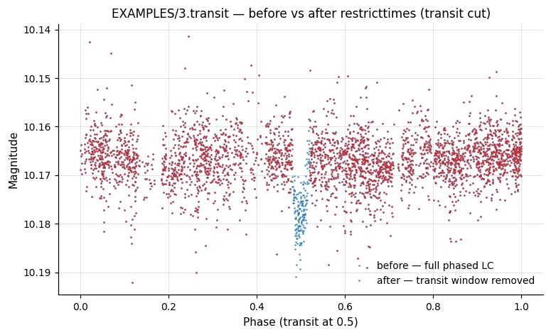
For a phase-folded illustration, the next figure shows EXAMPLES/3.transit phased on its BLS period before and after using -restricttimes expr to remove the in-transit points:
-SYSREM
Syntax
-SYSREM
    Ninput_color ["column" col1]
    Ninput_airmass initial_airmass_file
    sigma_clip1 sigma_clip2 saturation correctlc
    omodel [model_outdir] otrends [trend_outfile]
    useweights
Description
Run the SYSREM PCA-like algorithm to identify and remove ensemble trends from a set of light curves. SYSREM iteratively fits a small number of "color"-like (per-star) and "airmass"-like (per-image) terms to the residuals. This command requires a light-curve list and automatically sets the -readall option.
Python equivalent: SYSREM.
Parameters
| Parameter | Description |
|---|---|
Ninput_color |
Number of initial "color"-like (per-star) trends; values are read from the input light-curve list. |
"column" col1 |
Column in the input list for the first color term (subsequent terms follow in order). |
Ninput_airmass |
Number of initial "airmass"-like (per-image) trends. |
initial_airmass_file |
File with the initial airmass trends. Column 1: JD; subsequent columns: trend values. |
sigma_clip1 |
σ-clipping for computing mean magnitudes. |
sigma_clip2 |
σ-clipping for determining which points contribute to the airmass/color terms. |
saturation |
Magnitudes brighter than this value do not contribute to the fit. |
correctlc |
1 to subtract the model from each LC, 0 to compute without subtracting. |
omodel [outdir] |
1 to write per-LC model files (suffix .sysrem.model; format JD mag mag_model sig clip). |
otrends [trend_outfile] |
1 to write the final trend signals (col 1: JD; subsequent cols: trend values). |
useweights |
Include this flag to weight observations by their formal uncertainties. |
Output columns: SYSREM_MeanMag_N, SYSREM_RMS_N.
References
Cite Tamuz, Mazeh & Zucker 2005, MNRAS, 356, 1466.
Examples
Example 1. Apply SYSREM to the light curves in EXAMPLES/trendlist_tfa. Two initial "color"-like terms (the second and third columns of the list) and one initial "airmass"-like term (taken from EXAMPLES/3) are used. 5σ clipping is applied for both the mean-magnitude calculation and the iterative fit; the saturation threshold is 8.0 mag. The model light curves are written to EXAMPLES/OUTDIR1, the converged trend vectors to EXAMPLES/OUTDIR1/sysrem.trends. The two -rms calls show the effect of SYSREM.
vartools -l EXAMPLES/trendlist_tfa -header \
    -rms \
    -SYSREM 2 1 EXAMPLES/3 5. 5. 8. 1 \
        1 EXAMPLES/OUTDIR1 1 EXAMPLES/OUTDIR1/sysrem.trends 1 \
    -rms
-TFA
Syntax
-TFA
    trendlist ["readformat" Nskip jdcol magcol]
    ["trend_coeff_priors" trend_coeff_prior_file
        ["use_lc_errors" | "weight_by_template_stddev"]]
    dates_file pixelsep ["xycol" xcol ycol]
    correctlc ocoeff [coeff_outdir] omodel [model_outdir]
    ["clip" sigclipfactor ["usemedian"] ["useMAD"]]
    ["fitmask" maskvar] ["outfitmask" outmaskvar]
    ["refmag" < value | "var" varname | "expr" expression > ["usemedian"]]
Description
Run the Trend Filtering Algorithm (TFA) on the light curves. TFA fits each light curve as a linear combination of a set of template (basis) light curves and subtracts the fit, yielding a filtered, detrended light curve. A light curve list (-l) is required, and the x and y pixel positions of each light curve must be available as columns in the list.
Python equivalent: TFA.
Parameters
| Parameter | Description |
|---|---|
trendlist |
File listing basis-vector files: trendname trendx trendy. ASCII or binary FITS. |
"readformat" Nskip jdcol magcol |
Format of the basis files (defaults: 0 1 2). |
"trend_coeff_priors" file |
Gaussian priors for trend coefficients (columns: trendname prior_mean prior_stddev). |
"use_lc_errors" |
Weight light-curve points by 1/err[i]. |
"weight_by_template_stddev" |
Weight points by 1/ave_template_stddev. |
dates_file |
File with the full set of JDs for all light curves (col 1: filename/id; col 2: JD). |
pixelsep |
Basis vectors within pixelsep of the target are excluded (avoids self-filtering). |
"xycol" xcol ycol |
Columns in the input list giving x and y positions (defaults: next two columns). |
correctlc |
1 to subtract the model from the LC; 0 to compute without subtracting. |
ocoeff [outdir] |
1 to write per-LC trend coefficients (suffix .tfa.coeff). |
omodel [outdir] |
1 to write the TFA model (suffix .tfa.model). |
"clip" sigclipfactor |
Outlier-clipping threshold before fitting (default: 5σ). Add "usemedian" and/or "useMAD" to change the reference statistic. |
"fitmask" maskvar |
Restrict points included in the trend fit (1 = include, 0 = exclude). The model is still evaluated and subtracted at excluded points. |
"outfitmask" outmaskvar |
Store the post-clipping fit mask in this variable. |
"refmag" < value \| "var" varname \| "expr" expression > |
Reset the level of the corrected light curve to a reference magnitude (requires correctlc=1). A uniform offset is added to every point so the mean of the corrected LC equals the value. The value may be a fixed number, a per-LC variable (var), or a per-LC analytic expression (expr). |
"usemedian" (after refmag) |
Set the median rather than the mean of the corrected LC to the reference magnitude. |
Output columns: TFA_MeanMag_N (out-of-fit mean magnitude), TFA_RMS_N (post-filter RMS).
References
Cite Kovács, Bakos and Noyes 2005, MNRAS, 356, 557.
Examples
Example 1. Apply TFA to the light curves in EXAMPLES/lc_list_tfa (the only LC there is EXAMPLES/3.transit). Use the trend templates in EXAMPLES/trendlist_tfa; the second and third columns give x/y positions for each template (the explicit xycol keyword is shown for clarity, though it would be the default here). Trend stars within 25 pixels of the source are excluded. The corrected light curve is passed to subsequent commands; the TFA coefficients and model are not written.
vartools -l EXAMPLES/lc_list_tfa -oneline -rms \
    -TFA EXAMPLES/trendlist_tfa EXAMPLES/dates_tfa \
        25.0 xycol 2 3 1 0 0
Example 2. Same as Example 1, but reset the level of the corrected light curve to a reference magnitude of 12.0. With refmag the corrected light curve is shifted by a constant so that its mean becomes 12.0 (TFA_MeanMag_1 reports 12.00000); adding usemedian would instead place the median at 12.0. The shift does not change the RMS.
vartools -l EXAMPLES/lc_list_tfa -oneline -rms \
    -TFA EXAMPLES/trendlist_tfa EXAMPLES/dates_tfa \
        25.0 xycol 2 3 1 0 0 refmag 12.0
-TFA_SR
Syntax
-TFA_SR
    trendlist ["readformat" Nskip jdcol magcol] dates_file
    ["decorr" iterativeflag Nlcterms lccolumn1 lcorder1 ...]
    pixelsep ["xycol" colx coly]
    correctlc ocoeff [coeff_outdir] omodel [model_outdir]
    dotfafirst tfathresh maxiter
    < "bin" nbins
            ["period" < "aov" | "ls" | "bls" | "list" ["column" col] | "fix" period >]
        | "signal" filename
        | "harm" Nharm Nsubharm
            ["period" < "aov" | "ls" | "bls" | "list" ["column" col] | "fix" period >] >
    ["clip" sigclipfactor ["usemedian"] ["useMAD"]]
    ["fitmask" maskvar] ["outfitmask" outmaskvar]
    ["refmag" < value | "var" varname | "expr" expression > ["usemedian"]]
Description
Run TFA in Signal Reconstruction (SR) mode. TFA-SR iteratively applies TFA and fits a signal model to the light curve, allowing the algorithm to preserve astrophysical signal that would otherwise be partially filtered out by plain TFA. Most parameters are identical to -TFA; the SR-specific parameters and the signal-model alternatives are described below.
Python equivalent: TFA_SR.
Parameters (in addition to those of -TFA)
| Parameter | Description |
|---|---|
"decorr" iterativeflag Nlcterms lccolumn1 lcorder1 ... |
Simultaneously decorrelate against Nlcterms light-curve-specific signals. iterativeflag=1 iterates between decorrelation and TFA (faster); iterativeflag=0 does both jointly (more correct, slower). |
dotfafirst |
1 = apply TFA first each iteration, then fit signal to residual; 0 = subtract signal first, then apply TFA. |
tfathresh |
Iteration stops when the fractional RMS change falls below this. |
maxiter |
Iteration cap. |
"bin" nbins |
Signal model = mean binned LC with nbins bins. Use optional "period" to phase-fold first. |
"signal" filename |
Signal model read from a file (a list of per-LC signal files). Fits a·signal + b. |
"harm" Nharm Nsubharm |
Signal model = Fourier series with Nharm harmonics + Nsubharm sub-harmonics. No iteration is required when using harm. Use "period" to specify the period source (aov, ls, bls, list, or fixed). |
"refmag" < value \| "var" varname \| "expr" expression > ["usemedian"] |
Reset the level of the corrected light curve to a reference magnitude (requires correctlc=1), exactly as for -TFA. With usemedian the median rather than the mean is set to the value. |
Output columns: TFA_SR_MeanMag_N, TFA_SR_RMS_N.
References
Cite Kovács, Bakos and Noyes 2005, MNRAS, 356, 557.
Examples
Example 1. Signal-reconstruction TFA with a harmonic signal model. We process light curves in EXAMPLES/lc_list_tfa_sr_harm (only EXAMPLES/2). -LS finds the period; we then save a copy of the light curve and use -Killharm + -rms to measure the signal amplitude and the residual RMS. After restoring the LC we run -TFA (no SR), measure the signal amplitude and residual RMS again — note the amplitude is lower because non-reconstructive TFA filters signal as well as noise. Restoring once more, we then apply -TFA_SR with harm mode using 0 harmonics and 0 sub-harmonics (a sine fit) and the period from -LS. The TFA coefficients and TFA model are written to EXAMPLES/OUTDIR1. After -TFA_SR the signal amplitude is comparable to the input value while the residual RMS is lower.
vartools -l EXAMPLES/lc_list_tfa_sr_harm -oneline -rms \
    -LS 0.1 10. 0.1 1 0 \
    -savelc \
    -Killharm ls 0 0 0 \
    -rms -restorelc 1 \
    -TFA EXAMPLES/trendlist_tfa EXAMPLES/dates_tfa \
        25.0 xycol 2 3 1 0 0 \
    -Killharm ls 0 0 0 \
    -rms -restorelc 1 \
    -TFA_SR EXAMPLES/trendlist_tfa EXAMPLES/dates_tfa \
        25.0 xycol 2 3 1 \
        1 EXAMPLES/OUTDIR1 1 EXAMPLES/OUTDIR1 \
        0 0.001 100 harm 0 0 period ls \
    -o EXAMPLES/OUTDIR1 nameformat 2.test_tfa_sr_harm \
    -Killharm ls 0 0 0 \
    -rms -restorelc 1
Example 2. Same idea as Example 1, but use phase-binning to define the signal instead of a harmonic series. Here -aov is used for the period, 5 higher-order harmonics are included in -Killharm (better for the non-sinusoidal starspot signal), and the iteration parameters (dotfafirst=0, tfathresh=0.001, maxiter=100) matter — TFA-SR alternates between binning the LC to define the signal and re-running TFA on the residual. We also process EXAMPLES/3.starspot along with EXAMPLES/2.
vartools -l EXAMPLES/lc_list_tfa_sr_bin -oneline -rms \
    -aov Nbin 20 0.1 10. 0.1 0.01 1 0 \
    -savelc \
    -Killharm aov 5 0 0 \
    -rms -restorelc 1 \
    -TFA EXAMPLES/trendlist_tfa EXAMPLES/dates_tfa \
        25.0 xycol 2 3 1 0 0 \
    -Killharm aov 5 0 0 \
    -rms -restorelc 1 \
    -TFA_SR EXAMPLES/trendlist_tfa EXAMPLES/dates_tfa \
        25.0 xycol 2 3 1 \
        1 EXAMPLES/OUTDIR1 1 EXAMPLES/OUTDIR1 \
        0 0.001 100 bin 100 period aov \
    -o EXAMPLES/OUTDIR1 nameformat %s.test_tfa_sr_bin \
    -Killharm aov 5 0 0 \
    -rms -restorelc 1
Example 3. Simultaneous decorrelation against a light-curve-specific trend (the JD column, fit to 2nd order). Setting iterativeflag=0 makes TFA-SR fit the LC-specific trend and the TFA templates jointly (more correct, but slower for large batches). The signal model is binning in time (bin 100, no period keyword). The before/after -decorr + -rms pair shows that TFA-SR does not suppress the signal and reduces the residual RMS.
vartools -l EXAMPLES/lc_list_tfa_sr_decorr -oneline -rms \
    -savelc \
    -decorr 1 1 1 0 1 1 2 0 \
    -rms -restorelc 1 \
    -TFA EXAMPLES/trendlist_tfa EXAMPLES/dates_tfa \
        25.0 xycol 2 3 1 0 0 \
    -decorr 1 1 1 0 1 1 2 0 \
    -rms -restorelc 1 \
    -TFA_SR EXAMPLES/trendlist_tfa EXAMPLES/dates_tfa \
        decorr 0 1 1 2 \
        25.0 xycol 2 3 1 \
        1 EXAMPLES/OUTDIR1 1 EXAMPLES/OUTDIR1 \
        0 0.001 100 bin 100 \
    -o EXAMPLES/OUTDIR1 nameformat %s.test_tfa_sr_decorr \
    -decorr 1 1 1 0 1 1 2 0 \
    -rms -restorelc 1