Light Curve Manipulation
This page documents the VARTOOLS commands that transform, filter, reformat, or inspect light curves. Commands are applied in the order given on the command line; each receives the (possibly modified) output of the previous command.
-binlc
Syntax
-binlc <"average" | "median" | "weightedaverage">
    <"binsize" <"var" bsvar | "expr" bsexpr | binsize> | "nbins" <"var" nbvar |
    "expr" nbexpr | nbins>>
    ["bincolumns" var1[:stats1][,var2[:stats2],...]]
    ["T0"
        <"fix" T0val | "var" varname | "list" ["column" col] | "fixcolumn"
        <colname | colnum> |
         "expr" expression>]
    ["binshift" <"var" bsvar | "expr" bsexpr | binshift>]
    <"tcenter" | "taverage" | "tmedian" | "tnoshrink" ["bincolumnsonly"]>
    ["maskpoints" maskvar]
Description
Bin the light curve in time (or in phase if a -Phase command has already been applied). All light curve vectors are binned together by default.
Python equivalent: binlc.
Parameters
| Parameter | Description |
|---|---|
average / median / weightedaverage |
Statistic used to combine points in a bin. Legacy integers 0, 1, 2 are also accepted. |
"binsize" binsize |
Bin width in units of the time (or phase) coordinate. |
"nbins" nbins |
Number of equal-width bins to divide the time span into. |
"bincolumns" var1[:stats1],... |
Override the binning statistic for specific named columns. Statistic names follow -stats conventions. |
"T0" ... |
Start time of the first bin. Sources: "fix" (command-line value), "list" (input list column), "fixcolumn" (prior output column), or "expr" (analytic expression). |
"binshift" binshift |
Shift the first bin start by t0 - binshift*binsize, where binshift is a dimensionless fraction of the binwidth (canonical use 0 <= binshift < 1; binshift=0.5 produces a half-bin shift). |
"tcenter" |
Output time for each bin is the bin center. |
"taverage" |
Output time is the average of times in the bin. |
"tmedian" |
Output time is the median of times in the bin. |
"tnoshrink" |
Replace every point with its binned value without reducing the length of the light curve. Append "bincolumnsonly" to restrict replacement to explicitly listed columns. |
"maskpoints" maskvar |
Only include points with maskvar > 0 in the binning. Masked-out points still receive the binned value when tnoshrink is active. |
Examples
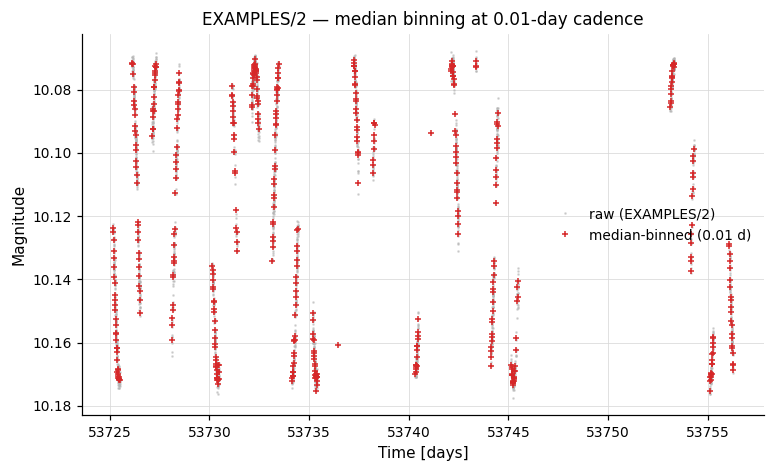
Example 1. Median-bin EXAMPLES/2 in time with a bin width of 0.01 days.
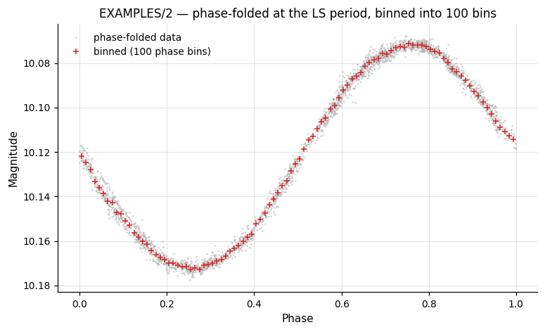
Example 2. Run an LS period search, phase-fold on the best period, then bin the phased light curve into 100 equal phase bins.
vartools -i EXAMPLES/2 \
    -LS 0.1 10.0 0.1 1 0 \
    -Phase ls \
    -binlc median nbins 100 tcenter \
    -o EXAMPLES/OUTDIR1/2.phasebin.txt
-changeerror
Syntax
Description
Replace the formal per-point measurement uncertainties in the light curve with the RMS of the light curve. This is useful when formal errors are unavailable or unreliable.
Python equivalent: changeerror.
Parameters
| Parameter | Description |
|---|---|
"maskpoints" maskvar |
Restrict the RMS calculation to points with maskvar > 0. |
Examples
Example 1. Replace formal errors with the light curve RMS and verify that χ²/dof becomes ≈ 1.
Output:
Name                = EXAMPLES/4
Chi2_0              =      5.19874
Weighted_Mean_Mag_0 =  10.35137
Mean_Mag_1          =  10.35142
RMS_1               =   0.00209
Npoints_1           =  3227
Chi2_2              =      1.00031
Weighted_Mean_Mag_2 =  10.35142
-converttime
Syntax
-converttime
    < "input" < "mjd" | "jd" | "hjd" | "bjd" > >
    ["inputsubtract" value] ["inputsys-tdb" | "inputsys-utc"]
    < "output" < "mjd" | "jd" | "hjd" | "bjd" > >
    ["outputsubtract" value] ["outputsys-tdb" | "outputsys-utc"]
    ["radec" < "list" ["column" col] | "fix" raval decval |
              "expr" raexpr decexpr | "perJD expr" raexpr decexpr |
              "perJD fromlc" ralccol declccol >
        ["epoch" epoch]]
    ["ppm" < "list" ["column" col] | "fix" mu_ra mu_dec >]
    ["input-radec" ...]
    ["input-ppm" ...]
    ["ephemfile" file] ["leapsecfile" file] ["planetdatafile" file]
    ["observatory" < code | "show-codes" >
      | "coords" ["xyz"]
          < "fix" lat lon alt | "list" [...] | "expr" [...] |
            "fromlc" col col col | "lcexpr" [...] >]
Description
Convert the time system of the light curve between Modified Julian Date (MJD), Julian Date (JD), Heliocentric Julian Date (HJD), and Barycentric Julian Date (BJD). BJD conversion requires VARTOOLS to be linked to the JPL NAIF cspice library. The internal precision near J2000.0 is approximately 0.1 milliseconds.
Python equivalent: converttime.
Parameters
| Parameter | Description |
|---|---|
"input" <system> |
Specify the input time system: "mjd", "jd", "hjd", or "bjd". |
"inputsubtract" value |
Constant subtracted from the stored input times (e.g. 2400000 if input is HJD-2400000). |
"inputsys-utc" / "inputsys-tdb" |
Whether input JDs were computed from UTC (default, typical for ground-based observatory headers) or from TDB (requires cspice). |
"output" <system> |
Desired output time system. |
"outputsubtract" value |
Subtract a constant from the output times. |
"radec" ... |
Source for the RA/Dec coordinates needed for HJD or BJD conversion. Options: "list", "fix" ra dec, "expr", "perJD expr" (per-observation expression), "perJD fromlc" (columns in the light curve). Coordinates in degrees; default epoch J2000.0. |
"ppm" ... |
Proper motion in mas/yr (RA, Dec). |
"input-radec" / "input-ppm" |
Separate RA/Dec and proper motion used for the input time system, if it differs from the target. |
"observatory" code |
Observatory code (use "show-codes" to list). |
"coords" ... |
Specify observer latitude (deg), longitude (deg E), altitude (m); or XYZ coordinates in the J2000 frame with "xyz". |
"ephemfile" / "leapsecfile" / "planetdatafile" |
JPL NAIF kernel files for BJD/TDB conversions. Can also be set via environment variables CSPICE_EPHEM_FILE, CSPICE_LEAPSEC_FILE, CSPICE_PLANETDATA_FILE. |
Examples
Example 1. Convert a light curve from JD to HJD given RA/Dec coordinates, subtracting 2400000 from the input JD.
vartools -i EXAMPLES/1 -quiet \
    -converttime input jd inputsubtract 2400000. output hjd \
    radec fix 88.079166 32.5533 \
    -o EXAMPLES/OUTDIR1/1.hjd
Example 2. Convert from UTC timestamps to Barycentric Julian Date in the TDB reference frame, requiring CSPICE kernel files and an observatory specification.
Requires CSPICE kernel files
This example reads the kernel file paths from the environment variables
CSPICE_EPHEM_FILE, CSPICE_LEAPSEC_FILE, and CSPICE_PLANETDATA_FILE.
Install the kernel files and set these variables as described in the
CSPICE kernel files section before
running.
vartools -i EXAMPLES/1.UTC -quiet \
    -inputlcformat t:1:utc:'%Y-%M-%DT%h:%m:%s',mag:2,err:3 \
    -converttime input jd inputsys-utc output bjd outputsys-tdb \
    radec fix 88.079166 32.5533 \
    ephemfile "${CSPICE_EPHEM_FILE}" \
    leapsecfile "${CSPICE_LEAPSEC_FILE}" \
    planetdatafile "${CSPICE_PLANETDATA_FILE}" \
    observatory flwo \
    -o EXAMPLES/OUTDIR1/1.bjd_tdb
-difffluxtomag
Syntax
-difffluxtomag <"var" mcvar | "expr" mcexpr | mag_constant>
    <"var" offvar | "expr" offexpr | offset> ["magcolumn" col]
Description
Convert a light curve from ISIS image-subtraction differential flux to magnitudes. Requires a light curve list (-l) where the reference magnitude of each star (after aperture correction) is provided as an additional column. The conversion formula is:
This command produces no statistics output to stdout; call -rms or -chi2 separately if statistics are needed.
Python equivalent: difffluxtomag.
Parameters
| Parameter | Description |
|---|---|
mag_constant |
Magnitude corresponding to a flux of 1 ADU. |
offset |
Additive constant applied to the output magnitudes. |
"magcolumn" col |
Column in the input list containing the reference magnitude. Default: next available column. |
Examples
Example 1. Convert ISIS differential fluxes to magnitudes. The reference magnitude (10.085) is piped via stdin as the second column of the list.
Output:
Example 2. Same as Example 1, but explicitly specify that the reference magnitude is in column 2.
-ensemblerescalesig
Syntax
Description
Rescale magnitude uncertainties across an ensemble of light curves by fitting a linear relation between E(rms)² and χ²·E(rms)² for all light curves, where E(rms) is the expected RMS based on the photometric uncertainties. The result is that χ²/dof is distributed about unity across the ensemble. Requires a list input; all light curves are read into memory.
The output includes the average rescale factor for each light curve, defined as sqrt(chi2_after / chi2_before).
Python equivalent: ensemblerescalesig.
Parameters
| Parameter | Description |
|---|---|
sigclip |
Sigma-clipping factor used to reject outliers in the ensemble χ² distribution. |
"maskpoints" maskvar |
Restrict the χ²/dof and expected RMS calculation to points with maskvar > 0. |
Examples
Example 1. Transform magnitude uncertainties across an ensemble of light curves, using -chi2 before and after to demonstrate the rescaling effect.
Output: table with columns Name, Chi2_0, Weighted_Mean_Mag_0, SigmaRescaleFactor_1, Chi2_2, Weighted_Mean_Mag_2 for EXAMPLES/1 through EXAMPLES/10.
-expr
Syntax
Description
Evaluate an analytic expression and assign the result to a named variable. If the variable does not yet exist it is created as a per-observation light-curve vector by default. The optional keywords change the variable type:
| Keyword | Variable type | Description |
|---|---|---|
| (none) | Per-observation | One value per point in the light curve (default). |
listvar |
Per-star | One value per light curve in the input list. Persists across all LCs. LC vectors on the RHS are evaluated at the first observation (index 0). |
scalar |
Per-thread | One value per processing thread. |
const |
Global constant | Single scalar value, same for all LCs. |
If the variable already exists, its type is preserved regardless of the keyword.
The optional outputcolumn trailing keyword exposes the LHS variable's computed value as a column in the result table (named Expr_<varname>_<command-index>). It is only valid when one of listvar, scalar, or const was given — for the default per-observation type the value would be one-per-observation rather than a single column, so outputcolumn raises a parse-time error in that case. This is equivalent to chaining a separate -print command but keeps the command index unchanged.
The expression can reference any existing light curve vectors (t, mag, err, other named columns), scalars from prior commands, or output columns identified by their header names. The expression engine supports aggregate functions like mean(mag), stddev(mag, t>53730), pct(mag, 95.0), etc. See the Analytic Expressions reference for the full list of supported operators, scalar functions, aggregate functions, and constants.
Python equivalent: expr.
Parameters
| Parameter | Description |
|---|---|
var |
Name of the variable to create or update. Cannot be an output-column name. |
expression |
Any analytic expression supported by the VARTOOLS expression evaluator. |
outputcolumn |
Optional flag (no value). Promotes the LHS variable to a result-table column. Only valid with listvar/scalar/const. |
Example
# Convert magnitudes to linear flux and store as a new column
vartools -i EXAMPLES/2 -expr 'flux=10^(-0.4*(mag-25.0))' -rms -oneline

# Compute per-star mean magnitude using an aggregate function
vartools -l EXAMPLES/lc_list -expr listvar 'avg=mean(mag)' -oneline

# Same as above, but expose the per-star mean as the result column Expr_avg_0
vartools -l EXAMPLES/lc_list -expr listvar 'avg=mean(mag)' outputcolumn -oneline

# Compute mean of only bright observations (mag < 10)
vartools -i EXAMPLES/2 -expr listvar 'bright_avg=mean(mag, mag<10)' -oneline

# Define a global constant
vartools -l EXAMPLES/lc_list -expr const 'zp=25.0' -expr 'flux=10^(-0.4*(mag-zp))' -oneline
Examples
Example 1. Add a constant to all magnitude values and then take the square root.
Input (first 3 lines of EXAMPLES/1):
Output (first 3 lines of EXAMPLES/1.add):
Example 2. Fit a sinusoid signal to each light curve and subtract it only when the delta chi² improvement is significant.
vartools -l EXAMPLES/lc_list -header \
    -LS 0.1 10. 0.1 1 0 \
    -rms -chi2 \
    -expr 'mag2=mag' \
    -harmonicfilter ls 0 0 0 \
    -rms -chi2 \
    -expr \
        'mag=(Npoints_5*(Chi2_6-Chi2_2)<-10000)*mag+
            (Npoints_5*(Chi2_6-Chi2_2)>=-10000)*mag2' \
    -o EXAMPLES/OUTDIR1 nameformat '%s.cleanharm'
Example 3. Convert magnitudes to fluxes with -expr, compute the median flux, then normalize by the median.
vartools -i EXAMPLES/1 \
    -expr 'flux=10^(-0.4*(mag-25.0))' \
    -stats flux median \
    -expr 'flux=flux/STATS_flux_MEDIAN_1' \
    -stats flux,mag median,stddev \
    -oneline
Output:
Name                = EXAMPLES/1
STATS_flux_MEDIAN_1 = 842674.79516438092
STATS_flux_MEDIAN_3 = 1
STATS_flux_STDDEV_3 = 0.1290865428119792
STATS_mag_MEDIAN_3  = 10.18585
STATS_mag_STDDEV_3  = 0.15946976931434606
-FFT
Syntax
Description
Compute the Fast Fourier Transform of a light curve vector using the GSL function gsl_fft_complex_forward(). The input and output vectors follow the standard GSL complex layout where element k corresponds to frequency k/(N·Δ) (for k < N/2) or negative frequencies (for k > N/2), where Δ is the assumed uniform time step between points and N is the number of points.
Use "NULL" for either input component to substitute a zero vector. Use "NULL" for either output component to discard that component.
Python equivalent: FFT.
Parameters
| Parameter | Description |
|---|---|
input_real_var |
Name of the light curve vector holding the real part of the input signal, or "NULL". |
input_imag_var |
Name of the light curve vector holding the imaginary part, or "NULL". |
output_real_var |
Variable name to store the real part of the transform, or "NULL". |
output_imag_var |
Variable name to store the imaginary part of the transform, or "NULL". |
Examples
Example 1. High-pass Fourier filter a uniformly sampled time-series by computing the FFT, zeroing low-frequency components, and applying the inverse FFT.
vartools -i EXAMPLES/11 \
    -FFT mag NULL fftreal fftimag \
    -rms \
    -expr \
      'fftreal=(NR>(Npoints_1/500.0))*(NR<(Npoints_1*499.0/500.0))*fftreal' \
    -expr \
      'fftimag=(NR>(Npoints_1/500.0))*(NR<(Npoints_1*499.0/500.0))*fftimag' \
    -IFFT fftreal fftimag mag_filter NULL \
    -o EXAMPLES/11.highpassfftfilter columnformat t,mag_filter
Output:
Example 2. Apply FFT-based high-pass and low-pass filtering to a non-uniformly sampled light curve by resampling to a uniform grid before transforming, then resampling back to the original time base.
vartools -i EXAMPLES/2 \
    -resample splinemonotonic gaps percentile_sep 80 bspline \
    -FFT mag NULL fftreal fftimag \
    -rms \
    -expr 'fftreal1=(NR>(Npoints_2/10.0))*(NR<(Npoints_2*9.0/10.0))*fftreal' \
    -expr 'fftimag1=(NR>(Npoints_2/10.0))*(NR<(Npoints_2*9.0/10.0))*fftimag' \
    -IFFT fftreal1 fftimag1 mag_filter NULL \
    -expr 'fftreal2=fftreal-((NR>(Npoints_2/10.0))*(NR<(Npoints_2*9.0/10.0))*fftreal)' \
    -expr 'fftimag2=fftimag-((NR>(Npoints_2/10.0))*(NR<(Npoints_2*9.0/10.0))*fftimag)' \
    -IFFT fftreal2 fftimag2 mag_filter2 NULL \
    -resample linear file fix EXAMPLES/2 column 1 \
    -expr 'mag_filter=mag_filter+Mean_Mag_2' \
    -o EXAMPLES/2.fftfilter columnformat t,mag_filter,mag_filter2,mag
Output:
-IFFT
Syntax
Description
Compute the Inverse Fast Fourier Transform of a light curve vector using the GSL function gsl_fft_complex_backward(). The parameter conventions are identical to those of -FFT, with input treated as frequency-domain data and output as time-domain data.
Python equivalent: IFFT.
Parameters
Same as -FFT. See above.
Examples
Example 1. High-pass Fourier filter a uniformly sampled time-series using -FFT and -IFFT in combination.
vartools -i EXAMPLES/11 \
    -FFT mag NULL fftreal fftimag \
    -rms \
    -expr \
      'fftreal=(NR>(Npoints_1/500.0))*(NR<(Npoints_1*499.0/500.0))*fftreal' \
    -expr \
      'fftimag=(NR>(Npoints_1/500.0))*(NR<(Npoints_1*499.0/500.0))*fftimag' \
    -IFFT fftreal fftimag mag_filter NULL \
    -o EXAMPLES/11.highpassfftfilter columnformat t,mag_filter
Output:
Example 2. Apply high-pass and low-pass filtering to a non-uniformly sampled light curve by resampling to a uniform grid, transforming with -FFT, filtering frequency components, and inverting with -IFFT.
vartools -i EXAMPLES/2 \
    -resample splinemonotonic gaps percentile_sep 80 bspline \
    -FFT mag NULL fftreal fftimag \
    -rms \
    -expr 'fftreal1=(NR>(Npoints_2/10.0))*(NR<(Npoints_2*9.0/10.0))*fftreal' \
    -expr 'fftimag1=(NR>(Npoints_2/10.0))*(NR<(Npoints_2*9.0/10.0))*fftimag' \
    -IFFT fftreal1 fftimag1 mag_filter NULL \
    -expr 'fftreal2=fftreal-((NR>(Npoints_2/10.0))*(NR<(Npoints_2*9.0/10.0))*fftreal)' \
    -expr 'fftimag2=fftimag-((NR>(Npoints_2/10.0))*(NR<(Npoints_2*9.0/10.0))*fftimag)' \
    -IFFT fftreal2 fftimag2 mag_filter2 NULL \
    -resample linear file fix EXAMPLES/2 column 1 \
    -expr 'mag_filter=mag_filter+Mean_Mag_2' \
    -o EXAMPLES/2.fftfilter columnformat t,mag_filter,mag_filter2,mag
Output:
-fluxtomag
Syntax
Description
Convert light curve flux values to magnitudes. The conversion is:
This command produces no output to stdout.
Python equivalent: fluxtomag.
Parameters
| Parameter | Description |
|---|---|
mag_constant |
Magnitude of a source with a flux of 1 ADU. |
offset |
Additive constant applied to the output magnitudes. |
Examples
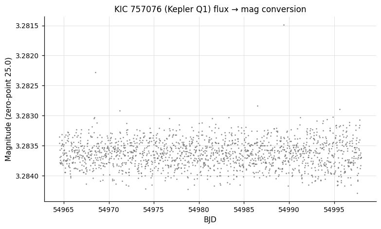
Example 1. Convert a Kepler public Q1 light curve from flux to magnitudes using a zero-point of 25.0 (1 ADU = magnitude 25).
vartools -i EXAMPLES/kplr000757076-2009166043257_llc.fits \
    -readformat 0 1 10 11 \
    -fluxtomag 25.0 0 \
    -o EXAMPLES/OUTDIR1/kplr000757076-2009166043257_llc.asc.txt
-magtoflux
Syntax
Description
Convert light curve magnitudes to fluxes. This is the inverse of -fluxtomag. The conversion is:
mag_constant is the magnitude of a source with a flux of 1 ADU. NaN and Inf inputs propagate to the output.
Alternatively, give the keyword normalize in place of mag_constant. In normalize mode, the fluxes are computed with an arbitrary internal zero-point and then both the flux array and the flux uncertainty array are divided by the median flux (NaNs rejected), so the output light curve has a median flux of 1. The output is then independent of the choice of zero-point. Useful when the absolute zero-point is unknown or unimportant — e.g. when subsequent commands only care about relative variability.
This command produces no output to stdout.
Python equivalent: magtoflux.
Parameters
| Parameter | Description |
|---|---|
mag_constant |
Magnitude of a source with a flux of 1 ADU. |
normalize (keyword) |
If given in place of mag_constant, normalize fluxes to median 1. |
Examples
Example 1. Round-trip with -fluxtomag on EXAMPLES/2 — RMS is preserved before and after.
Example 2. Normalize EXAMPLES/2 to a median flux of 1 and report basic statistics.
-match
Syntax
-match
    < "file" filename | "inlist" inlistcolumn >
    ["opencommand" command] ["skipnum" Nskip]
    ["skipchar" <skipchar1[,skipchar2,...]>] ["delimiter" delimiter]
    < "matchcolumn" < varname:column | colnum > >
    < "addcolumns" varname1:colnum1[:coltype1[:colformat1]]
        [,varname2:colnum2[:coltype2[:colformat2]],...] >
    < "cullmissing" | "nanmissing" | "missingval" value >
Description
Perform a row-by-row match of an external data file to the light curve, merging columns from the file into the light curve. The match is performed on a specified variable (by default the time t). Float/double columns are matched within the tolerance set by -jdtol; all other types are matched exactly.
Python equivalent: match.
Parameters
| Parameter | Description |
|---|---|
"file" filename |
A single file matched to every light curve. Files ending in .fits are treated as binary FITS tables. |
"inlist" col |
Read the name of the match file for each light curve from column col of the input list. |
"opencommand" command |
Shell command to pre-process each match file; %s is replaced with the filename. Output is read from the command's stdout. |
"skipnum" Nskip |
Number of lines to skip at the top of each match file. |
"skipchar" chars |
Comma-separated list of comment characters (default: #). |
"delimiter" delim |
Column delimiter (default: whitespace). |
"matchcolumn" varname:colnum |
Light-curve variable and match-file column number (or FITS column name) to use as the match key. |
"addcolumns" varname:colnum[:type[:fmt]],... |
Columns to merge from the match file into the light curve. New variables are created; existing ones are overwritten. |
"cullmissing" |
Remove light curve rows that have no match. |
"nanmissing" |
Set unmatched rows to NaN (float/double) or 0 (integer/string). |
"missingval" value |
Set unmatched rows to the specified value. |
Examples
Example 1. Join EXAMPLES/1 with the file EXAMPLES/dates_tfa, matching on the time column. The default tolerance for matching different times is set by -jdtol. The imagename string from the first column of dates_tfa is added to the light curve as a new column. Because we used cullmissing, rows in EXAMPLES/1 with no match are removed. The light curve including the new imagename column is then written to EXAMPLES/1_withID.txt.
vartools -i EXAMPLES/1 -inputlcformat t:1,mag:2,err:3 \
    -match file EXAMPLES/dates_tfa matchcolumn t:2 \
        addcolumns imagename:1:string cullmissing \
    -o EXAMPLES/1_withID.txt columnformat imagename,t,mag,err
The first few rows of the output file:
M37.0.0167.fits 53725.173920000001 10.085000000000001 0.0011900000000000001
M37.0.0168.fits 53725.17654 10.0847 0.0014400000000000001
M37.0.0169.fits 53725.17772 10.0825 0.00123
M37.0.0170.fits 53725.179409999997 10.081 0.0011900000000000001
M37.0.0171.fits 53725.180789999999 10.081899999999999 0.0013500000000000001
-Phase
Syntax
-Phase <"aov" | "ls" | "bls" | "fixcolumn" <colname | colnum>
        | "list" ["column" col] | "fix" period
        | "var" varname | "expr" expression>
    ["T0" <"bls" phaseTc | "fixcolumn" <colname | colnum>
        | "list" ["column" col] | "fix" T0
        | "var" varname | "expr" expression>]
    ["phasevar" var] ["startphase" startphase]
Description
Replace the time axis of the light curve with its phase and sort by phase. The phase is defined as ((t - T0) mod P) / P, running from 0 to 1 (or from startphase to startphase + 1). After -Phase, time-based binning commands like -binlc operate in phase space.
Python equivalent: Phase.
Parameters
| Parameter | Description |
|---|---|
"aov" |
Use the best period from the most recent -aov or -aov_harm command. |
"ls" |
Use the best period from the most recent -LS command. |
"bls" |
Use the best period from the most recent -BLS command. |
"fixcolumn" col |
Use the value of a previously computed output column (by name or number). |
"list" |
Read the period from the input list (optionally specify the "column"). |
"fix" P |
Fix the period to the value P for all light curves. |
"T0" ... |
Reference epoch for phase zero. "bls" phaseTc assigns the BLS mid-transit time the phase phaseTc; other sources follow standard vartools conventions. Default: the earliest time in the light curve. |
"phasevar" var |
Store phases in the variable var instead of overwriting t. |
"startphase" startphase |
Start of the phase range (default 0; range becomes [startphase, startphase+1)). |
Examples
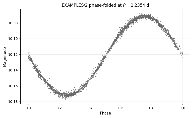
Example 1. Phase-fold the light curve on a fixed period of 1.2354 days and write the result to disk.
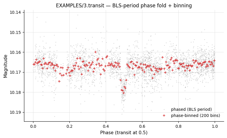
Example 2. Detect a transit with BLS, phase-fold on the BLS period placing mid-transit at phase 0.5, write the phase-folded light curve, then median-bin it into 200 phase bins.
vartools -i EXAMPLES/3.transit -oneline \
    -BLS q 0.01 0.1 0.5 5.0 20000 200 7 1 0 0 0 \
    -Phase bls T0 bls 0.5 \
    -o EXAMPLES/OUTDIR1/3.phase.txt \
    -binlc median nbins 200 tcenter \
    -o EXAMPLES/OUTDIR1/3.phasebin.txt
-resample
Syntax
-resample
    < "nearest" | "linear" | "spline" ["left" yp1] ["right" ypn]
      | "splinemonotonic" | "bspline" ["nbreaks" nbreaks] ["order" order] >
    ["file" < "fix" times_file ["column" col] |
              "list" ["listcolumn" col] ["tcolumn" col] > |
     ["tstart" < "fix" val | "fixcolumn" col | "list" | "expr" expr >]
     ["tstop"  < "fix" val | "fixcolumn" col | "list" | "expr" expr >]
     ["delt"   < "fix" val | "fixcolumn" col | "list" | "expr" expr > |
      "Npoints" < "fix" val | "fixcolumn" col | "list" | "expr" expr >]]
    ["gaps" <separation spec> <method>]
    ["extrap" <method>]
Description
Resample the light curve onto a new time base by interpolating all light curve vectors. The default output grid runs from the first to the last observed time with a step equal to the minimum observed time separation. String-type columns (e.g. image IDs) are always resampled with the "nearest" method.
Python equivalent: resample.
Parameters
| Parameter | Description |
|---|---|
"nearest" |
Nearest-neighbor (step-function) interpolation. |
"linear" |
Linear interpolation. |
"spline" |
Cubic spline interpolation. Optional "left"/"right" set boundary first-derivative conditions. |
"splinemonotonic" |
Cubic spline constrained to be monotonic between observations. |
"bspline" |
Basis-spline interpolation. Optional "nbreaks" (default 15) and "order" (default 3). If nbreaks < 2, breaks are increased until χ²/dof ≤ 1 (can be slow). |
"file" ... |
Specify an arbitrary (non-uniform) time base from a file. |
"tstart" / "tstop" / "delt" / "Npoints" |
Override the start, stop, step size, or total number of resampled points. Each accepts "fix", "fixcolumn", "list", or "expr". |
"gaps" <sep> <method> |
Use a different interpolation method for points that are farther than sep from any observed time. Separation can be fixed, taken from a column, or derived from the data distribution ("frac_min_sep", "frac_med_sep", "percentile_sep"). |
"extrap" <method> |
Use a different method for extrapolated points (beyond the observed time range). |
Examples
Example 1. Resample using linear interpolation with default time sampling.
Example 2. Resample using monotonic spline between fixed start/stop times with exactly 1000 output points.
vartools -i EXAMPLES/2 -resample splinemonotonic \
    tstart fix 53726 tstop fix 53756 Npoints fix 1000 \
    -o EXAMPLES/2.resample.example2
Example 3. Resample EXAMPLES/4 onto the time grid of EXAMPLES/8 using linear interpolation.
Example 4. Resample onto a uniform 0.001-day grid, using a B-spline for normal gaps, nearest-neighbour for large gaps (> 80th-percentile separation), and nearest-neighbour for extrapolation.
vartools -i EXAMPLES/1 -resample splinemonotonic \
    tstart fix 53725 tstop fix 53757 delt fix 0.001 \
    gaps percentile_sep 80 bspline nbreaks 15 order 3 \
    extrap nearest \
    -o EXAMPLES/1.resample.example4
-rescalesig
Syntax
Description
Rescale the magnitude uncertainties of each light curve independently so that χ²/dof = 1 for that light curve. The rescale factor applied to each light curve is included in the output table. Unlike -ensemblerescalesig, this operates per-light-curve without fitting an ensemble relation.
Python equivalent: rescalesig.
Parameters
| Parameter | Description |
|---|---|
"maskpoints" maskvar |
Restrict the χ²/dof calculation to points with maskvar > 0. |
Examples
Example 1. Rescale the formal errors in a light curve so that χ²/dof equals 1, demonstrating the effect with -chi2 before and after.
Output:
Name                  = EXAMPLES/4
Chi2_0                = 5.19874
Weighted_Mean_Mag_0   = 10.35137
SigmaRescaleFactor_1  = 0.43858
Chi2_2                = 1.00000
Weighted_Mean_Mag_2   = 10.35137
-sortlc
Syntax
Description
Sort the light curve. By default it is sorted by time. If any subsequent command requires time-sorted data and the light curve was re-sorted by another variable, it will be automatically re-sorted by time at the start of that command.
Python equivalent: sortlc.
Parameters
| Parameter | Description |
|---|---|
"var" varname |
Sort by this named variable instead of time. |
"reverse" |
Sort in descending order. |
Examples
Example 1. Sort EXAMPLES/2 in reverse time order (most recent first) and write the result to disk.
Example 2. Sort EXAMPLES/2 by magnitude (brightest first). The var keyword names the variable to sort by.