Transit search and fit
Detrend with TFA and then search for transits with BLS using a trapezoidal
in-transit fit. The input is EXAMPLES/3.transit, the LC created by the
transit injection example.
Command line
./vartools -l EXAMPLES/lc_list_tfa \
    -rms \
    -TFA EXAMPLES/trendlist_tfa EXAMPLES/dates_tfa 25.0 1 0 0 \
    -BLS density 1.41 0.5 2.0 0.5 5.0 optimal 0.1 200 7 2 0 1 EXAMPLES/OUTDIR1 1 fittrap \
    -rms \
    -oneline
Name                         = EXAMPLES/3.transit
Mean_Mag_0                   =  10.16727
RMS_0                        =   0.00542
Expected_RMS_0               =   0.00104
Npoints_0                    =  3417
TFA_MeanMag_1                =  10.16714
TFA_RMS_1                    =   0.00471
BLS_Period_1_2               =     2.12402761
BLS_Tc_1_2                   = 53727.294878968052
BLS_SN_1_2                   =  69.00454
BLS_SDE_1_2                  =   4.41122
BLS_Depth_1_2                =   0.01186
BLS_Qtran_1_2                =   0.03586
BLS_Qingress_1_2             =   0.16670
BLS_Npointsintransit_1_2     =   161
BLS_Ntransits_1_2            =     4
BLS_SignaltoPinknoise_1_2    =  15.93733
BLS_Period_2_2               =     1.35229047
...
RMS_3                        =   0.00405
Python
import pyvartools as vt
from pyvartools import commands as cmd

pipe = (vt.Pipeline()
        .rms()
        .TFA(
            trendlist="EXAMPLES/trendlist_tfa",
            dates_file="EXAMPLES/dates_tfa",
            pixelsep=25.0,
            correct_lc=True,
            save_coeffs=False,
            save_model=False,
        )
        .BLS(
            density_mode=True,
            stellar_density=1.41,        # solar density, g/cm³
            min_exp_dur_frac=0.5,
            max_exp_dur_frac=2.0,
            minper=0.5, maxper=5.0,
            subsample=0.1,               # oversampling for "optimal" grid
            nbins=200,
            timezone=7, npeaks=2,
            save_periodogram=False,
            correct_lc=True,
            fittrap=True,
        )
        .rms())

result = pipe.run_filelist("EXAMPLES/lc_list_tfa")

row = result.vars.iloc[0]
for col in ["RMS_0", "TFA_RMS_1", "BLS_Period_1_2", "BLS_Tc_1_2",
            "BLS_SN_1_2", "BLS_SDE_1_2", "BLS_Depth_1_2",
            "BLS_Qtran_1_2", "BLS_SignaltoPinknoise_1_2",
            "BLS_Period_2_2", "RMS_3"]:
    print(f"{col:<30} = {row[col]}")
RMS_0                          = 0.00542
TFA_RMS_1                      = 0.00471
BLS_Period_1_2                 = 2.12402761
BLS_Tc_1_2                     = 53727.29487896805
BLS_SN_1_2                     = 69.00454
BLS_SDE_1_2                    = 4.41122
BLS_Depth_1_2                  = 0.01186
BLS_Qtran_1_2                  = 0.03586
BLS_SignaltoPinknoise_1_2      = 15.93733
BLS_Period_2_2                 = 1.35229047
RMS_3                          = 0.00405
Notes
-TFA fits a linear combination of template trend light curves to remove
shared systematics. The template list is EXAMPLES/trendlist_tfa (paths +
pixel coordinates for each star); EXAMPLES/dates_tfa is the global cadence
file. The 25.0 is the minimum pixel separation between target and template
— templates within 25 pixels of EXAMPLES/3.transit are excluded, so the
target's own signal can't leak back into the detrending model. The three
final flags are correctlc=1 save_coeffs=0 save_model=0.
-BLS then searches for transits on the detrended LC:
density 1.41 0.5 2.0— stellar density (g/cm³) plus min/max fractional scaling of the expected transit duration; BLS computes the per-trial-period duration bounds from the density assuming a circular orbit.0.5 5.0— period range in days.optimal 0.1— optimal frequency grid with a subsampling factor of 0.1 (finer than the native optimal spacing by 10×).200— phase bins.7— local timezone offset in hours (used for the one-night-fraction statistic).2— number of peaks to report.0 1 EXAMPLES/OUTDIR1— skip periodogram output, write the BLS model LC to the output dir.1 fittrap— subtract the best-fit box before passing to the next command, and fit a trapezoidal transit at each peak (which adds theQingressandOOTmagcolumns).
The final -rms captures the residual scatter after the transit model is
subtracted. For this LC the RMS drops from 0.00542 mag (raw) to 0.00471 mag
(post-TFA) to 0.00405 mag (post-TFA + transit removal). The best BLS period,
2.12403 d, matches the injected 2.12345 d; the 1.352 d secondary peak is a
harmonic alias.
BLS_SignaltoPinknoise is the most useful single-statistic indicator for
transit candidates; values above ~10 are strong candidates once the LC has
been properly detrended.
Variation: Mandel-Agol fit at the BLS period
After BLS finds a candidate, we seed a Mandel-Agol physical transit fit
with the BLS period, transit center, depth, and fractional duration; the
initial impact parameter is 0.1. ophcurve writes the fitted model as a
phase curve from −0.5 to 0.5 so it can be overplotted directly on the
folded observations.
./vartools -i EXAMPLES/3.transit \
    -BLS density 1.41 0.5 2.0 0.5 5.0 optimal 0.1 200 7 1 0 0 0 fittrap \
    -MandelAgolTransit \
        expr BLS_Period_1_0 expr BLS_Tc_1_0 \
        expr 'sqrt(BLS_Depth_1_0)' expr '1.0/(BLS_Qtran_1_0*pi)' \
        b 0.1 0.0 0.0 -1 quad 0.3 0.3 \
        1 1 1 1 0 0 1 0 0 0 0 0 \
        ophcurve EXAMPLES/OUTDIR1 -0.5 0.5 0.001 \
    -oneline
expr BLS_Period_1_0 etc. pull the BLS outputs from the prior command
into the MA init values; b 0.1 initializes the impact parameter (which
is what the fit varies, via fitinclterm=1). mconst0 = -1 tells
vartools to estimate the out-of-transit magnitude from the light curve.
Name                         = EXAMPLES/3.transit
BLS_Period_1_0               =     2.12402761
BLS_Tc_1_0                   = 53727.294970417119
BLS_SN_1_0                   =  66.76648
BLS_SDE_1_0                  =   4.34232
BLS_Depth_1_0                =   0.01139
BLS_Qtran_1_0                =   0.03603
BLS_SignaltoPinknoise_1_0    =  13.48275
...
MandelAgolTransit_Period_1   =     2.12339179
MandelAgolTransit_T0_1       = 53727.29676768
MandelAgolTransit_r_1        =   0.09810
MandelAgolTransit_a_1        =   9.66412
MandelAgolTransit_bimpact_1  =   0.27251
MandelAgolTransit_inc_1      =  88.38413
MandelAgolTransit_mconst_1   =  10.16686
MandelAgolTransit_chi2_1     =  27.06389
The Python equivalent mirrors the CLI: expressions reference the BLS
output columns, bimpact=0.1 is the initial impact parameter, and
save_phcurve=True with ophcurve_phmin/phmax/phstep captures the
fitted model as a DataFrame. A cmd.Phase(...) step after the fit
folds the observations on the MA-optimized ephemeris and stores the
per-point phase in a new LC vector ph_obs, which is picked up directly
by cmd.o(capture=True).
import matplotlib
matplotlib.use("Agg")
import matplotlib.pyplot as plt
import pyvartools as vt
from pyvartools import commands as cmd

lc = vt.LightCurve.from_file("EXAMPLES/3.transit")

result = (vt.Pipeline()
        .BLS(
            density_mode=True, stellar_density=1.41,
            min_exp_dur_frac=0.5, max_exp_dur_frac=2.0,
            minper=0.5, maxper=5.0,
            subsample=0.1, nbins=200,
            timezone=7, npeaks=1,
            save_periodogram=False, correct_lc=False, fittrap=True,
        )
        .MandelAgolTransit(
            P0="expr BLS_Period_1_0",
            T00="expr BLS_Tc_1_0",
            r0="expr sqrt(BLS_Depth_1_0)",
            a0="expr 1.0/(BLS_Qtran_1_0*pi)",
            bimpact=0.1,
            mconst0=-1,                  # let vartools estimate the baseline
            ld_coeffs=[0.3, 0.3],
            fitephem=1, fitr=1, fita=1, fitinclterm=1,
            fite=0, fitomega=0, fitmconst=1, fitldcoeffs=[0, 0],
            save_phcurve=True,
            ophcurve_phmin=-0.5, ophcurve_phmax=0.5, ophcurve_phstep=0.001,
        )
        .Phase(
            period="fixcolumn MandelAgolTransit_Period_1",
            T0="fixcolumn MandelAgolTransit_T0_1",
            phasevar="ph_obs",
            startphase=-0.5,
        )
        .o(capture=True, key="folded")).run(lc)

fit    = result.varobjs.MandelAgolTransit
folded = result.files["folded"].to_dataframe()
model  = result.files["MandelAgolTransit_phcurve_1"]

fig, ax = plt.subplots(figsize=(7, 3.5))
ax.plot(folded["ph_obs"], folded["mag"], ".", ms=1.5,
        color="0.6", label="observed")
ax.plot(model[0], model[1], "-", lw=1.3,
        color="C3", label="Mandel-Agol fit")
ax.set_xlim(-0.15, 0.15)
ax.invert_yaxis()
P, T0 = float(fit.Period), float(fit.T0)
ax.set_xlabel(f"Phase  (P = {P:.6f} d, T0 = {T0:.5f})")
ax.set_ylabel("mag")
ax.legend(loc="lower right")
fig.tight_layout()
fig.savefig("/tmp/mandel_agol_fit.png", dpi=120)

for name, val in [("P", float(fit.Period)),
                  ("T0", float(fit.T0)),
                  ("r", float(fit.r)),
                  ("a/R*", float(fit.a)),
                  ("bimpact", float(fit.bimpact)),
                  ("inc", float(fit.inc)),
                  ("mconst", float(fit.mconst)),
                  ("chi2", float(fit.chi2))]:
    print(f"{name:<8} = {val}")
P        = 2.12339179
T0       = 53727.29676768
r        = 0.0981
a/R*     = 9.66412
bimpact  = 0.27251
inc      = 88.38413
mconst   = 10.16686
chi2     = 27.06389
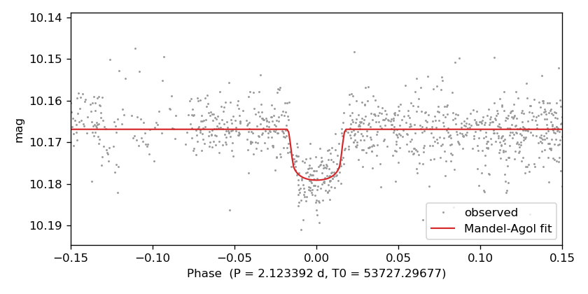
The fitted period (2.12339 d) shifts by ~0.9 minutes from the BLS grid
value (2.12403 d) and the fitted T0 (BJD 53727.29677) by ~2.6 minutes
from the BLS transit centre. The red curve is the Mandel-Agol model
written by ophcurve (directly on a [−0.5, 0.5] phase grid); the gray
points are the observations folded on the fitted ephemeris via
cmd.Phase(..., phasevar="ph_obs", startphase=-0.5).
Variation: GPU transit search with CETRA
CETRA (Smith et al. 2025, MNRAS, 539, 297) is a CUDA-accelerated transit-detection algorithm that can operate faster than the CPU-based BLS algorithm. Because it's a Python package rather than a vartools command, it enters into the pipeline through cmd.python(inprocess=True) — the in-process callback runs the user code in pyvartools' own interpreter, so import cetra (and the PyCUDA context it initializes) sees the same GPU resources as the calling script.
Once CETRA finds the period / T0 / duration, the rest of the pipeline is the same chain as the BLS variant above: BLSFixPerDurTc re-derives depth and other transit statistics at the CETRA ephemeris, then MandelAgolTransit fits a Mandel-Agol model.
Requires CUDA + PyCUDA + CETRA
This variation needs an NVIDIA GPU, the CUDA toolkit on PATH (so pycuda can compile kernels), and the cetra Python package in the same conda env as pyvartools. See the CETRA README for installation.
import numpy as np
import pyvartools as vt
import cetra
import matplotlib.pyplot as plt


def cetra_search(t, mag, mag_err):
    """Run CETRA on a magnitude LC, return the highest-SNR Transit object."""
    fluxes = 10.0 ** (-0.4 * mag)
    flux_errors = fluxes * mag_err / 1.0857
    medflux = float(np.median(fluxes))
    fluxes /= medflux
    flux_errors /= medflux
    lc_cetra = cetra.LightCurve(t, fluxes, flux_errors)
    td = cetra.TransitDetector(lc_cetra)
    td.linear_search()
    td.period_search()
    return td.get_max_snr_periodic_transit()


lc = vt.LightCurve.from_file("EXAMPLES/3.transit")

result = (vt.Pipeline()
          .python(
              "tr = cetra_search(t, mag, err); "
              "period   = float(tr.period); "
              "t0       = float(tr.t0); "
              "duration = float(tr.duration)",
              invars="t,mag,err",
              outvars="period,t0,duration",
              outputcolumns="period,t0,duration",
              inprocess=True)
          .BLSFixPerDurTc(period="period", duration="duration", Tc="t0",
                          correct_lc=False, fittrap=True)
          .MandelAgolTransit(
              P0="expr BLSFixPerDurTc_Period_1",
              T00="expr BLSFixPerDurTc_Tc_1",
              r0="expr sqrt(BLSFixPerDurTc_Depth_1)",
              a0="expr 1.0/(BLSFixPerDurTc_Qtran_1*pi)",
              bimpact=0.1, mconst0=-1,
              ld_coeffs=[0.3, 0.3],
              fitephem=1, fitr=1, fita=1, fitinclterm=1,
              fite=0, fitomega=0, fitmconst=1, fitldcoeffs=[0, 0])
          ).run(lc, capture_lc=True)

P  = float(result.vars["MandelAgolTransit_Period_2"])
T0 = float(result.vars["MandelAgolTransit_T0_2"])
print(f"CETRA period         = {result.vars['PYTHON_period_0']:.6f} d")
print(f"Mandel-Agol P        = {P:.6f} d")
print(f"Mandel-Agol T0       = {T0:.5f}")
print(f"Mandel-Agol r        = {result.vars['MandelAgolTransit_r_2']:.5f}")
print(f"Mandel-Agol a/R*     = {result.vars['MandelAgolTransit_a_2']:.4f}")
print(f"Mandel-Agol inc      = {result.vars['MandelAgolTransit_inc_2']:.3f} deg")
print(f"Mandel-Agol chi2     = {result.vars['MandelAgolTransit_chi2_2']:.3f}")

# Phase-fold the (untransformed) LC at the fitted Mandel-Agol ephemeris.
out = result.lc
ph = ((out.t - T0) / P)
ph -= np.floor(ph)
ph[ph > 0.5] -= 1.0

fig, ax = plt.subplots(figsize=(7, 4))
ax.plot(ph, out.mag, ".", ms=2, color="0.4")
ax.set_xlim(-0.15, 0.15)
ax.invert_yaxis()
ax.set_xlabel(f"Phase  (P = {P:.6f} d, T0 = {T0:.5f})")
ax.set_ylabel("mag")
ax.set_title("CETRA → BLSFixPerDurTc → Mandel-Agol")
fig.tight_layout()
fig.savefig("/tmp/cetra_transit_fold.png", dpi=120)
CETRA period         = 2.123535 d
Mandel-Agol P        = 2.123393 d
Mandel-Agol T0       = 53727.29676
Mandel-Agol r        = 0.09774
Mandel-Agol a/R*     = 9.9821
Mandel-Agol inc      = 89.153 deg
Mandel-Agol chi2     = 27.065
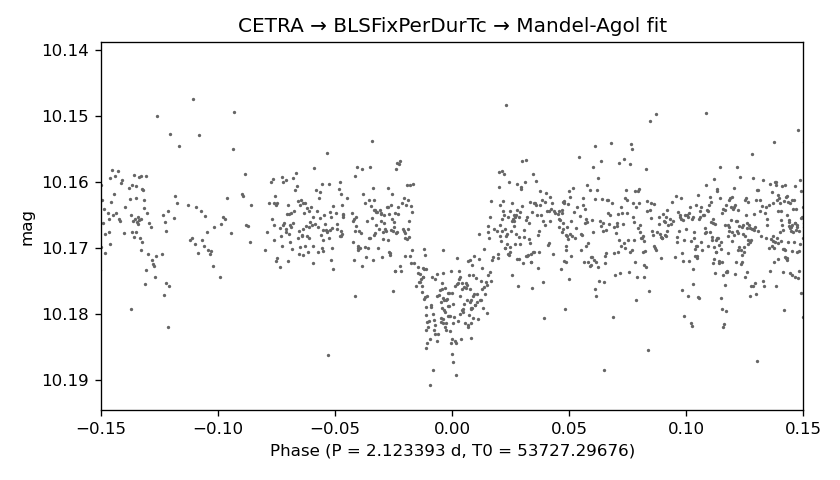
CETRA's grid period (2.1235 d) is within ~10 s of the Mandel-Agol fitted period (2.12339 d) — close enough that BLSFixPerDurTc finds the transit cleanly, and the subsequent Mandel-Agol fit produces parameters consistent with the BLS-seeded variant above (r = 0.098, a/R* = 9.98, i = 89.15°).
Variation: high-pass detrending + CETRA + fit
CETRA is designed for detrended light curves, so a quick way to improve robustness on noisier data is to remove a few low-frequency Fourier modes first. Setting period=10.0 with nharm=0 and nsubharm=10 on cmd.harmonicfilter fits and subtracts the fundamental at 10 d plus sub-harmonics at 20, 30, …, 110 d — i.e. a high-pass that removes any structure on timescales ≥ 10 d while leaving the ~2 d transit signal alone.
import numpy as np
import pyvartools as vt
import cetra
import matplotlib.pyplot as plt


def cetra_search(t, mag, mag_err):
    fluxes = 10.0 ** (-0.4 * mag)
    flux_errors = fluxes * mag_err / 1.0857
    medflux = float(np.median(fluxes))
    fluxes /= medflux
    flux_errors /= medflux
    lc_cetra = cetra.LightCurve(t, fluxes, flux_errors)
    td = cetra.TransitDetector(lc_cetra)
    td.linear_search()
    td.period_search()
    return td.get_max_snr_periodic_transit()


lc = vt.LightCurve.from_file("EXAMPLES/3.transit")

result = (vt.Pipeline()
          # High-pass at P=10 d: subtract the fundamental + 10 sub-harmonics
          # (covering periods 10, 20, …, 110 d).  nharm=0 → no harmonics
          # shorter than 10 d are removed, so the ~2 d transit stays intact.
          .harmonicfilter(period=10.0, nharm=0, nsubharm=10)
          .python(
              "tr = cetra_search(t, mag, err); "
              "period   = float(tr.period); "
              "t0       = float(tr.t0); "
              "duration = float(tr.duration)",
              invars="t,mag,err",
              outvars="period,t0,duration",
              outputcolumns="period,t0,duration",
              inprocess=True)
          .BLSFixPerDurTc(period="period", duration="duration", Tc="t0",
                          correct_lc=False, fittrap=True)
          .MandelAgolTransit(
              P0="expr BLSFixPerDurTc_Period_2",
              T00="expr BLSFixPerDurTc_Tc_2",
              r0="expr sqrt(BLSFixPerDurTc_Depth_2)",
              a0="expr 1.0/(BLSFixPerDurTc_Qtran_2*pi)",
              bimpact=0.1, mconst0=-1,
              ld_coeffs=[0.3, 0.3],
              fitephem=1, fitr=1, fita=1, fitinclterm=1,
              fite=0, fitomega=0, fitmconst=1, fitldcoeffs=[0, 0])
          ).run(lc, capture_lc=True)

P  = float(result.vars["MandelAgolTransit_Period_3"])
T0 = float(result.vars["MandelAgolTransit_T0_3"])
print(f"CETRA period         = {result.vars['PYTHON_period_1']:.6f} d")
print(f"Mandel-Agol P        = {P:.6f} d")
print(f"Mandel-Agol T0       = {T0:.5f}")
print(f"Mandel-Agol r        = {result.vars['MandelAgolTransit_r_3']:.5f}")
print(f"Mandel-Agol a/R*     = {result.vars['MandelAgolTransit_a_3']:.4f}")
print(f"Mandel-Agol inc      = {result.vars['MandelAgolTransit_inc_3']:.3f} deg")
print(f"Mandel-Agol chi2     = {result.vars['MandelAgolTransit_chi2_3']:.3f}")

# Phase-fold the (already detrended) LC at the fitted ephemeris.
out = result.lc
ph = ((out.t - T0) / P)
ph -= np.floor(ph)
ph[ph > 0.5] -= 1.0

fig, ax = plt.subplots(figsize=(7, 4))
ax.plot(ph, out.mag, ".", ms=2, color="0.4")
ax.set_xlim(-0.15, 0.15)
ax.invert_yaxis()
ax.set_xlabel(f"Phase  (P = {P:.6f} d, T0 = {T0:.5f})")
ax.set_ylabel("mag (after high-pass)")
ax.set_title("harmonicfilter (P=10d, nsubharm=10) → CETRA → Mandel-Agol")
fig.tight_layout()
fig.savefig("/tmp/cetra_highpass_transit_fold.png", dpi=120)
CETRA period         = 2.123535 d
Mandel-Agol P        = 2.123408 d
Mandel-Agol T0       = 53727.29540
Mandel-Agol r        = 0.09268
Mandel-Agol a/R*     = 10.3707
Mandel-Agol inc      = 89.097 deg
Mandel-Agol chi2     = 26.148
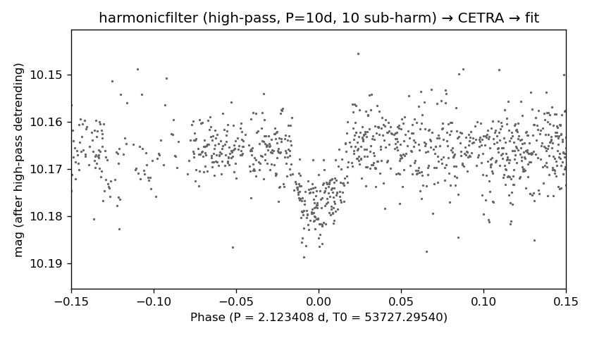
The high-pass step removes a small amount of long-timescale structure that BLS-style searches typically don't care about but that can bias a model fit; here the χ² drops modestly from 27.1 to 26.1, and the fitted radius / a /inclination shift by a fraction of their per-fit uncertainties — consistent with the picture that the input LC was already mostly clean.