Model Fitting
Commands for fitting analytic models to light curves, from simple harmonic series to full transit and microlensing models.
-linfit
-linfit function paramlist ["modelvar" varname]
    ["reject" <"var" scvar | "expr" scexpr | sigclip> ["useMAD"]
    ["iter" ["fixednum" number]]]
    ["correctlc"]
    ["omodel" model_outdir ["format" nameformat]]
    ["fitmask" maskvar]
Fit a function that is linear in its free parameters to each light curve using least squares.
Python equivalent: linfit.
Parameters
function— Analytic function to fit (e.g.,'a1*t^2+a2*t+a3').paramlist— Comma-separated list of free parameter names (e.g.,'a1,a2,a3'). Parameter names must not conflict with any existing vector variable names (t,mag,err, etc.)."modelvar" varname— Store the best-fit model in the vector variablevarnamefor use by later commands."reject" sigclip— Reject outliers beyondsigclipsigma and refit."useMAD"— Use the MAD statistic rather than the standard deviation when measuring scatter."iter"— Iteratively reject until no additional outliers are found."fixednum" number— Perform at mostnumberrejection iterations."correctlc"— Subtract the best-fit model from the light curve."omodel" model_outdir— Output the model tomodel_outdir. Default filename:model_outdir/basefilename.linfit.model. Use"format"keyword to override the naming convention."fitmask" maskvar— Only include points withmaskvar > 0in the fit.
Examples
Example 1. Fit a quadratic polynomial to a light curve. The minimum time value is first computed via -stats and stored as a reference point, then linear regression is performed using a normalized time variable to avoid numerical precision issues.
vartools -i EXAMPLES/1 \
    -stats t min \
    -expr t0=STATS_t_MIN_0 \
    -linfit 'a*(t-t0)^2+b*(t-t0)+c' 'a,b,c' \
    -oneline
Output:
Name          = EXAMPLES/1
STATS_t_MIN_0 = 53725.173920000001
Linfit_a_2    = 0.00025540627746042932
Linfit_erra_2 = 1.9561241332987699e-07
Linfit_b_2    = 0.0097933162509034055
Linfit_errb_2 = 5.9117874714733109e-06
Linfit_c_2    = 10.083037598482507
Linfit_errc_2 = 3.2584974556662493e-05
-nonlinfit
Syntax
-nonlinfit function paramlist ["linfit" linfitparams]
    ["errors" error_expr]
    ["covariance"
        <"squareexp" amp_var rho_var
         | "exp" amp_var rho_var
         | "matern" amp_var rho_var nu_var>]
    ["priors" priorlist] ["constraints" constraintlist]
    <"amoeba" ["tolerance" <"var" v | "expr" e | tol>]
              ["maxsteps" <"var" v | "expr" e | steps>]
     | "mcmc" ["Naccept" <"var" v | "expr" e | N>
              | "Nlinkstotal" <"var" v | "expr" e | N>]
            ["fracburnin" <"var" v | "expr" e | frac>]
            ["eps" <"var" v | "expr" e | eps>] ["skipamoeba"]
            ["chainstats" exprlist statslist]
            ["maxmemstore" maxmem]
            ["outchains" outdir ["format" format] ["printevery" N]] >
    ["modelvar" varname] ["correctlc"]
    ["omodel" model_outdir ["format" nameformat]]
Description
Fit a function that is nonlinear in its free parameters to each light curve. Two optimisers are supported: amoeba (downhill simplex / Nelder-Mead, fast greedy local minimisation) and mcmc (differential-evolution Markov chain Monte Carlo, full posterior exploration). Parameters that enter the model linearly may be moved out of the nonlinear search and fit by linear least squares (linfit), which is faster and more numerically stable. Optional Gaussian-process covariance kernels (squareexp, exp, matern) handle correlated errors; arbitrary priors and constraints can be added.
Python equivalent: nonlinfit.
Parameters
| Parameter | Description |
|---|---|
function |
Analytic function to fit (e.g. 'a*exp(-(t-t0)^2/2/sigma^2)+b'). |
paramlist |
Comma-separated free parameters with initial guesses and step sizes: var=init:step (e.g. 't0=5.0:2.0,sigma=10.0:8.0'). |
"linfit" linfitparams |
List of parameters that enter linearly; optimized by linear least squares. Not included in MCMC posteriors. |
"errors" error_expr |
Analytic expression for the per-point uncertainties used in the likelihood. |
"covariance" |
Gaussian-process kernel: "squareexp" amp ρ, "exp" amp ρ, or "matern" amp ρ ν. Linear-only fitting is not permitted with covariance. |
"priors" priorlist |
Comma-separated list of prior expressions, each evaluating to -2 ln P. Example: '(t0-4.0)^2/3.0^2' is a Gaussian prior on t0 with mean 4.0 and σ = 3.0. |
"constraints" constraintlist |
Comma-separated list of constraint expressions (e.g. 'sigma>0'). |
"amoeba" |
Use the downhill simplex (Nelder-Mead) optimiser. Sub-keywords: "tolerance" (Δχ² convergence threshold), "maxsteps" (cap). |
"mcmc" |
Use differential-evolution MCMC. Sub-keywords: "Naccept"/"Nlinkstotal", "fracburnin" (default 0.1), "eps" (default 0.001), "skipamoeba", "chainstats", "maxmemstore" (GB; default 4), "outchains" outdir. |
"modelvar" varname |
Store the best-fit model in light-curve vector varname. |
"correctlc" |
Subtract the best-fit model from the light curve. |
"omodel" model_outdir |
Write the model to a file (default suffix .nonlinfit.model). |
Output columns (suffix _N is the command index):
| Column | Description |
|---|---|
Nonlinfit_<param>_N |
Best-fit value of each non-linear parameter and (for linfit parameters) each linear coefficient. |
Nonlinfit_<param>_err_N |
1-σ uncertainty in each parameter. For amoeba these are derived from the covariance matrix at the optimum; for mcmc they are taken from the posterior. |
Nonlinfit_Chi2_N |
χ² of the best-fit model. |
Nonlinfit_Npts_N |
Number of light-curve points used in the fit. |
When mcmc is used with chainstats, additional columns are emitted following the supplied statslist (see -stats). When outchains is given, the full chain is written to outdir/<lcname>.mcmc.
Examples
Example 1. Inject a Gaussian into EXAMPLES/3 (with the third -expr call) and fit a Gaussian back to it. Two of the four parameters (c, the peak time, and d, the standard deviation) enter nonlinearly and are searched with the downhill-simplex (amoeba) algorithm; the linear amplitude (b) and offset (a) are recovered by linear least squares (linfit a,b). The model is written to EXAMPLES/OUTDIR1/3.nonlinfit.model.
vartools -i EXAMPLES/3 \
    -stats t min,max \
    -expr t1=STATS_t_MIN_0 \
    -expr 'Dt=(STATS_t_MAX_0-STATS_t_MIN_0)' \
    -expr 'mag=mag+0.1*exp(-0.5*((t-(t1+Dt*0.2))/(Dt*0.05))^2)' \
    -nonlinfit 'a+b*exp(-(t-c)^2/(2*d^2))' \
        'c=(t1+Dt*0.3):(0.1*Dt),d=(Dt*0.1):(0.1*Dt)' \
        linfit a,b amoeba omodel EXAMPLES/OUTDIR1/ \
    -oneline
Example 2. Same model and injection as Example 1, but explore the χ² landscape with MCMC. All four parameters (a, b, c, d) are now free non-linear parameters with their own initial guesses and step sizes. 10,000 chain links are written to EXAMPLES/OUTDIR1/3.mcmc.
vartools -i EXAMPLES/3 \
    -stats t min,max \
    -expr t1=STATS_t_MIN_0 \
    -expr 'Dt=(STATS_t_MAX_0-STATS_t_MIN_0)' \
    -expr 'mag=mag+0.1*exp(-0.5*((t-(t1+Dt*0.2))/(Dt*0.05))^2)' \
    -nonlinfit 'a+b*exp(-(t-c)^2/(2*d^2))' \
        'a=10.167:0.0002,b=0.1:0.0008,c=(t1+Dt*0.2):(0.005),d=(Dt*0.05):(0.016)' \
        mcmc Nlinkstotal 10000 outchains EXAMPLES/OUTDIR1/ \
    -oneline
-MandelAgolTransit
-MandelAgolTransit <bls | blsfixper
        | <"var" v | "expr" e | P0> <"var" v | "expr" e | T00>
          <"var" v | "expr" e | r0> <"var" v | "expr" e | a0>
          <"i" <"var" v | "expr" e | inclination> | "b" <"var" v | "expr" e |
          bimpact>>
          <"var" v | "expr" e | e0> <"var" v | "expr" e | omega0>
          <"var" v | "expr" e | mconst0>>
    <"quad" | "nonlin"> <"var" v | "expr" e | ldcoeff1_0>
        ... <"var" v | "expr" e | ldcoeffn_0> fitephem
    fitr fita fitinclterm fite fitomega fitmconst fitldcoeff1 ... fitldcoeffn
    fitRV [RVinputfile RVmodeloutfile <"var" v | "expr" e | K0>
    <"var" v | "expr" e | gamma0> fitK fitgamma]
    correctlc omodel [model_outdir] ["modelvar" var]
    ["ophcurve" curve_outdir phmin phmax phstep]
    ["ojdcurve" curve_outdir jdstep]
Fit a Mandel and Agol (2002) transit model to the light curve. Initial parameters can come from a preceding -BLS run or be entered directly.
Python equivalent: MandelAgolTransit.
Initial parameters (when not using "bls" or "blsfixper")
| Parameter | Description |
|---|---|
P0 |
Orbital period |
T00 |
Time of transit center |
r0 |
Ratio of planet radius to stellar radius (Rp/R★) |
a0 |
Ratio of semi-major axis to stellar radius (a/R★) |
"i" incl |
Inclination (degrees), or "b" bimp for impact parameter |
e0 |
Eccentricity |
omega0 |
Argument of periastron (degrees) |
mconst0 |
Out-of-transit magnitude (if negative, estimated from the data) |
Limb darkening
"quad"— Quadratic limb darkening; requires 2 coefficients."nonlin"— Non-linear (Claret) limb darkening; requires 4 coefficients.
Fit flags
fitephem fitr fita fitinclterm fite fitomega fitmconst fitldcoeff1 ... fitldcoeffn — Each is 1 to allow that parameter to vary, 0 to hold it fixed.
Optional radial velocity fitting
Set fitRV=1 to simultaneously fit an RV curve from RVinputfile (columns: JD, RV, RVerror). The model RV (evaluated at evenly spaced phase points) is written to RVmodeloutfile. Provide initial values K0 and gamma0 and flags fitK, fitgamma.
Output control
correctlc— Set to1to subtract the transit model from the light curve.omodel— Set to1to output the model; providemodel_outdir. Output suffix:.mandelagoltransit.model."modelvar" var— Store the best-fit model in vector variablevar."ophcurve" curve_outdir phmin phmax phstep— Output a model phase curve tocurve_outdirwith phases fromphmintophmaxin steps ofphstep. Suffix:.mandelagoltransit.phcurve."ojdcurve" curve_outdir jdstep— Output a model light curve evaluated at times spanning the observations with step sizejdstep. Suffix:.mandelagoltransit.jdcurve.
Citation: Mandel, K. & Agol, E. 2002, ApJ, 580, L171.
Examples
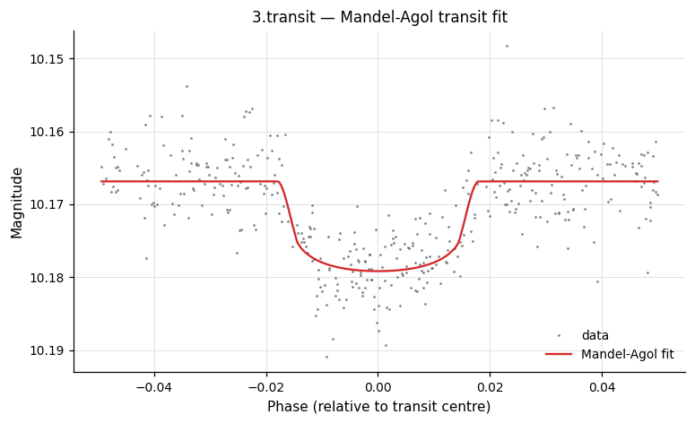
Example 1. Use -BLS to identify a transit signal in the light curve EXAMPLES/3.transit, then fit a Mandel-Agol transit model to it. A quadratic limb-darkening law is used with coefficients 0.3471 and 0.3180. The ephemeris (P and T0), Rp/R★, a/R★, and the impact parameter are varied; eccentricity and argument of periastron are held fixed.
vartools -i EXAMPLES/3.transit -oneline \
    -BLS q 0.01 0.1 0.5 5.0 20000 200 7 1 0 0 0 \
    -MandelAgolTransit bls quad 0.3471 0.3180 \
        1 1 1 1 0 0 1 0 0 0 0 1 EXAMPLES/OUTDIR1
Output:
BLS_Period_1_0              = 2.12312625
BLS_Tc_1_0                  = 53727.297046247397
MandelAgolTransit_Period_1  = 2.12328176
MandelAgolTransit_r_1       = 0.09789
MandelAgolTransit_bimpact_1 = 0.33094
MandelAgolTransit_chi2_1    = 27.06054
-SoftenedTransit
-SoftenedTransit
    < bls | blsfixper | P0 T00 eta0 delta0 mconst0 >
    cval0 fitP fitT0 fiteta fitcval fitdelta fitmconst
    correctlc omodel [model_outdir]
    fit_harm [< "aov" | "ls" | "bls"
            | "list" ["column" col] | "fix" Pharm >
        nharm nsubharm]
Fit a Protopapas, Jimenez and Alcock (2005) "softened" transit model to the light curve. Initial parameters may come from a preceding -BLS or -BLSFixPer run, or be entered directly.
Python equivalent: SoftenedTransit.
Parameters
P0,T00,eta0,delta0,mconst0— Initial period, time of transit, transit duration parameter, depth, and out-of-transit magnitude (use a negative value formconst0to estimate it from the data).cval0— Initial value for the softening parameter.fitP fitT0 fiteta fitcval fitdelta fitmconst— Flags (1to vary,0to hold fixed) for each parameter.correctlc— Set to1to subtract the model from the light curve.omodel— Set to1to output the model tomodel_outdir. Suffix:.softenedtransit.model.fit_harm— Set to1to simultaneously fit a harmonic series; specify the period source andnharm,nsubharm.
Citation: Protopapas, P., Jimenez, R. & Alcock, C. 2005, MNRAS, 362, 460.
Examples
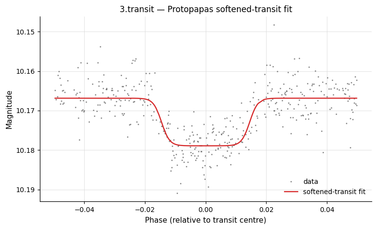
Example 1. Use -BLS to identify a transit signal in EXAMPLES/3.transit, then fit a Protopapas et al. 2005 softened transit model initialized from the BLS results. The ephemeris, eta, cval, delta, and mconst are varied; the model is not subtracted from the light curve.
vartools -i EXAMPLES/3.transit -oneline \
    -BLS q 0.01 0.1 0.5 5.0 20000 200 7 1 0 0 0 \
    -SoftenedTransit bls 1 1 1 1 1 0 1 EXAMPLES/OUTDIR1 0
Output:
Name = EXAMPLES/3.transit
BLS_Period_1_0               = 2.12312625
BLS_Tc_1_0                   = 53727.297046247397
BLS_SN_1_0                   = 38.39425
BLS_SR_1_0                   = 0.00237
BLS_SDE_1_0                  = 4.77204
BLS_Depth_1_0                = 0.01136
BLS_Qtran_1_0                = 0.03000
BLS_deltaChi2_1_0            = -24130.93833
BLS_Ntransits_1_0            = 4
BLS_Rednoise_1_0             = 0.00156
BLS_Whitenoise_1_0           = 0.00490
BLS_SignaltoPinknoise_1_0    = 12.89679
SoftenedTransit_Period_1     = 2.12322112
SoftenedTransit_T0_1         = 53727.29783160
SoftenedTransit_eta_1        = 0.06171206
SoftenedTransit_cval_1       = -10.87159958
SoftenedTransit_delta_1      = -0.01206461
SoftenedTransit_mconst_1     = 10.16686817
SoftenedTransit_chi2perdof_1 = 27.04335183
-microlens
-microlens
    ["f0"
        ["fix" fixval | "var" varname | "expr" expression
            | "list" ["column" col]
            | "fixcolumn" <colname | colnum>
            | "auto"]
        ["step" initialstepsize] ["novary"]]
    ["f1" ... ] ["u0" ... ] ["t0" ... ] ["tmax" ... ]
    ["correctlc"] ["omodel" outdir]
Fit a simple (Wozniak et al. 2001, AcA, 51, 175) microlensing model to the light curve using a downhill simplex optimizer.
Python equivalent: microlens.
Parameters
For each of the five model parameters (f0, f1, u0, t0, tmax), optionally specify:
"fix" fixval— Fix the initial value for all light curves."list" ["column" col]— Read the initial value from the input list."fixcolumn" <colname | colnum>— Use a previously computed statistic as the initial value."auto"— Automatically determine the initial value (default for all parameters)."step" initialstepsize— Initial step size for the downhill simplex."novary"— Hold this parameter fixed at its initial value.
Output control
"correctlc"— Subtract the best-fit model from the light curve."omodel" outdir— Output the model tooutdir. Output suffix:.microlens.
Citation: Wozniak, P.R. et al. 2001, AcA, 51, 175.
Examples
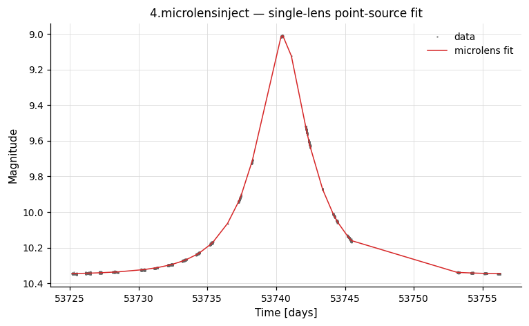
Example 1. Fit a simple microlensing model to the simulated light curve EXAMPLES/4.microlensinject. Initial values for all five parameters are set automatically, and the best-fit model is written to EXAMPLES/OUTDIR1/.
vartools -i EXAMPLES/4.microlensinject -oneline \
    -microlens f0 auto f1 auto u0 auto t0 auto tmax auto \
        omodel EXAMPLES/OUTDIR1
Output:
Name                   = EXAMPLES/4.microlensinject
Microlens_f0_0         = 7.242316197338e-05
Microlens_f1_0         = 7.5541525219661e-05
Microlens_u0_0         = 7.242316197338e-05
Microlens_t0_0         = 3.9109521538222
Microlens_tmax_0       = 53740.494617109
Microlens_chi2perdof_0 = 4.4674961258953
-Starspot
-Starspot
    <aov | ls | list ["column" col] | "fix" period
        | "var" varname | "expr" expression
        | "fixcolumn" <colname | colnum>>
    <"var" v | "expr" e | a0> <"var" v | "expr" e | b0>
    <"var" v | "expr" e | alpha0> <"var" v | "expr" e | i0>
    <"var" v | "expr" e | chi0> <"var" v | "expr" e | psi00>
    <"var" v | "expr" e | mconst0> fitP fita fitb
    fitalpha fiti fitchi fitpsi fitmconst correctlc omodel [model_outdir]
Deprecated
This command is deprecated as of VARTOOLS 1.3. Use the -macula extension command instead.
Fit a single, circular, uniform-temperature starspot model to the light curve using the Dorren (1987) model. Parameters a0, b0, alpha0, i0, chi0, psi00 are as defined in Dorren 1987. Set mconst0 negative to estimate it automatically from the data. Fit flags (fitP, fita, etc.) are 1 to vary and 0 to fix the corresponding parameter.
Python equivalent: Starspot.
Citation: Dorren 1987, ApJ, 320, 756.
Examples
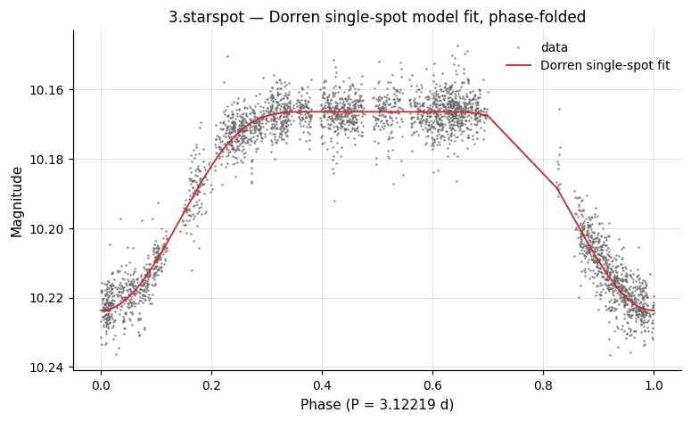
Example 1. Determine the rotation period via AOV analysis, then apply Dorren 1987 single-starspot modeling. Initial parameters: a=0.0298, b=0.08745, spot radius=20°, inclination=85°, latitude=30°, longitude=0°. The unspotted magnitude is estimated automatically. Period, spot radius, inclination, latitude, longitude, and magnitude are varied; a and b remain fixed. The best-fit model is output to EXAMPLES/OUTDIR1/.
vartools -i EXAMPLES/3.starspot -oneline \
    -aov Nbin 20 0.1 10. 0.1 0.01 5 0 \
    -Starspot aov 0.0298 0.08745 20. 85. 30. 0. -1 \
        1 0 0 1 1 1 1 1 0 1 EXAMPLES/OUTDIR1/
Output:
Name                   = EXAMPLES/3.starspot
Period_1_0             = 3.07960303
AOV_1_0                = 2861.35783
AOV_SNR_1_0            = 605.83431
AOV_NEG_LN_FAP_1_0    = 4755.85353
Starspot_Period_1      = 3.12218969
Starspot_a_1           = 0.02980
Starspot_b_1           = 0.08745
Starspot_alpha_1       = 22.51312
Starspot_inclination_1 = 69.03963
Starspot_chi_1         = 30.00411
Starspot_psi0_1        = 0.00000
Starspot_mconst_1      = 10.16641
Starspot_chi2perdof_1  = 26.58796
-decorr
-decorr
    correctlc zeropointterm subtractfirstterm
    Nglobalterms globalfile1 order1 ... globalfileN orderN
    Nlcterms lccolumn1 lcorder1 ... lccolumnN lcorderN
    omodel [modeloutdir] ["maskpoints" maskvar]
Deprecated
This command is deprecated as of VARTOOLS 1.3. Use -linfit instead.
Decorrelate the light curves against specified external or light-curve-specific signals using polynomial regression.
Python equivalent: decorr.
Parameters
correctlc—1to apply the decorrelation to the light curve;0to compute and output the coefficients and χ² without modifying the light curve.zeropointterm—1to include a zero-point offset term in the fit;0to omit it.subtractfirstterm—1to decorrelate against(signal - signal[0])rather thansignaldirectly (useful for detrending against JD).Nglobalterms— Number of global signal files.globalfile1 ... globalfileN— Names of global signal files (format:JD signal_value).order1 ... orderN— Polynomial orders for each global signal (must be ≥ 1).Nlcterms— Number of light-curve-specific signals.lccolumn1 ... lccolumnN— Column indices in the light curve for each light-curve-specific signal.lcorder1 ... lcorderN— Polynomial orders for each light-curve-specific signal.omodel—1to output the decorrelation model tomodeloutdir. Suffix:.decorr.model."maskpoints" maskvar— Optional. Only points withmaskvar > 0contribute to the fit.
Examples
Example 1. Fit quadratic polynomials to light curves using a JD-based light-curve term (column 1), including a zero-point offset, with the first term subtracted to reduce rounding errors. Report RMS before and after decorrelation.