Calling Python or R
Wrappers for vartools' embedded -python / -R interpreters, used to run user code on each light curve from within a pipeline.
R — Run R code
Syntax
cmd.R(command, fromfile=False, init=None, init_fromfile=False,
      vars=None, invars=None, outvars=None, outputcolumns=None,
      process_all_lcs=False, verbose=False, continueprocess=None)
Description
Execute arbitrary R code on each light curve. VARTOOLS embeds the user-supplied code in an R function and calls it once per light curve (or once for all light curves with process_all_lcs=True). Light-curve variables are passed to R as native R vectors. vars specifies variables to pass both into and out of R; invars/outvars allow separate control. init is R code run once before the batch loop begins (typically used for library imports and function definitions).
The R_HOME environment variable must be set before calling vartools (find the correct value with R RHOME; adding export R_HOME=$(R RHOME) to your .bashrc is recommended). Under -parallel, a separate R sub-process is launched per thread; initialization runs independently for each thread, and globals are not shared between threads.
CLI equivalent: -R.
Parameters
| Parameter | Type | Description |
|---|---|---|
command |
str |
Inline R code (default), or path to an R script file when fromfile=True. |
fromfile |
bool |
If True, treat command as a file path rather than an inline string. |
init |
str or None |
R code (or file path when init_fromfile=True) executed once before processing. Typical use: library imports and function definitions. |
init_fromfile |
bool |
If True, init is a file path. |
vars |
str or None |
Comma-separated list of variables passed both into and received back from R. |
invars |
str or None |
Variables passed into R only (alternative to vars). |
outvars |
str or None |
Variables received back from R only (alternative to vars). |
outputcolumns |
str or None |
Subset of out-vars to emit in the output statistics table as R_<name>_N. |
process_all_lcs |
bool |
Pass all light curves at once. Vector inputs arrive as lists of vectors; scalar inputs as lists. The output variables must also be lists with one entry per LC. |
verbose |
bool |
Allow R to print to stdout (default: R runs in --slave mode). |
continueprocess |
int or None |
Reuse the sub-process from the N-th prior -R (1-indexed). Shares R state; no initialization code may be supplied. |
Output
This command produces no output statistics by default; user-defined outputcolumns appear as R_<name>_N in result.vars.
Examples
Example 1. Compute the standard deviation of the magnitudes for each light curve in EXAMPLES/lc_list using R; the result appears as R_b_0 in the output table.
batch = (vt.Pipeline()
         .R("b <- sd(mag)",
            invars="mag", outvars="b", outputcolumns="b")
         ).run_filelist("EXAMPLES/lc_list",
                        perpoint_columns={"t": 1, "mag": 2, "err": 3})
print(batch.vars[["Name", "R_b_0"]])
Example 2. Same as Example 1 but using process_all_lcs=True to send the whole batch to R at once. Inside R, mag arrives as a list of vectors and the output b must also be a list (one entry per LC).
batch = (vt.Pipeline()
         .R("b <- list(); for(i in 1:length(mag)) "
            "{ b[[i]] <- sd(mag[[i]]); }",
            invars="mag", outvars="b", outputcolumns="b",
            process_all_lcs=True)
         ).run_filelist("EXAMPLES/lc_list",
                        perpoint_columns={"t": 1, "mag": 2, "err": 3})
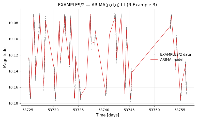
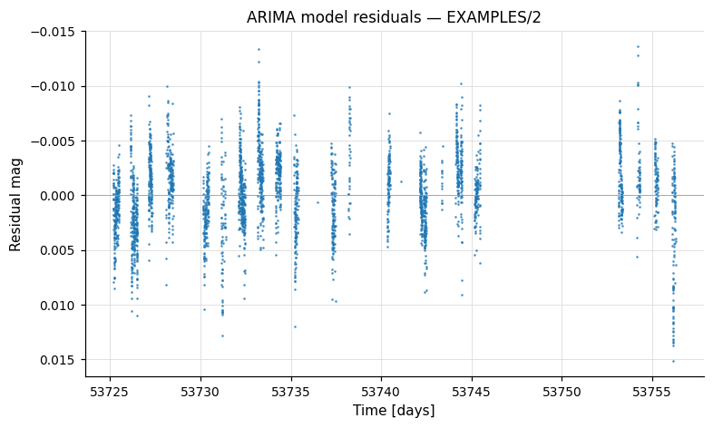
Example 3. ARIMA modelling using R's forecast package. After saving the original mag, we bin and resample the LC onto a uniform grid (ARIMA needs evenly-sampled data), call auto.arima, and subtract the residuals to obtain the smoothed model mag_arima. The model is then resampled back to the original time grid (using the list-form resample) and the original mag is restored. Requires tseries and forecast to be installed in R.
batch = (vt.Pipeline()
         .savelc()
         .binlc(method="average", binsize=0.05, time_output="taverage")
         .resample(method="linear", delt=0.05)
         .R(("mag_ts <- ts(mag, start=1, end=length(t), frequency=1); "
             "arima_model <- auto.arima(mag_ts); "
             "mag_arima <- mag - as.vector(arima_model$residuals);"),
            init="library(tseries); library(forecast);",
            invars="mag,t", outvars="mag_arima")
         .resample(method="linear",
                   file_times="list", list_column=1, t_column=1)
         .restorelc(1, vars="mag")
         .o(outdir="EXAMPLES/OUTDIR1",
            nameformat="%s.arimamodel",
            columnformat="t,mag,mag_arima")
         ).run_filelist("EXAMPLES/lc_list",
                        perpoint_columns={"t": 1, "mag": 2, "err": 3})
The resulting *.arimamodel files contain t, the original mag, and the smoothed mag_arima:
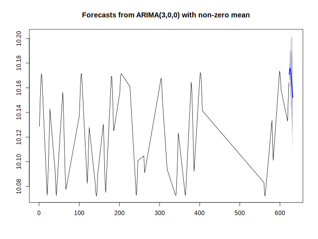
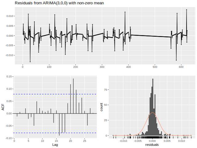
Example 4. Same as Example 3 but with the ARIMA fit + diagnostic plots wrapped in a function DoArimaFitPlot defined in EXAMPLES/Rexample4.R. A -python step strips the directory prefix off Name to get the per-LC basename (a stand-in for any place where Python's string handling is more convenient than R's), then -R is loaded with init_fromfile=True so the Rexample4.R definitions are read once and DoArimaFitPlot is called per LC. The function writes per-LC *.arimaforecast.png and *.arimaresiduals.png files via R's forecast plotting helpers.
batch = (vt.Pipeline()
         .savelc()
         .binlc(method="average", binsize=0.05, time_output="taverage")
         .resample(method="linear", delt=0.05)
         .python('lcbasename = Name.split("/")[-1]',
                 invars="Name", outvars="lcbasename")
         .R('mag_arima <- DoArimaFitPlot(mag, "EXAMPLES/OUTDIR1/", lcbasename)',
            init="EXAMPLES/Rexample4.R", init_fromfile=True,
            invars="mag,t,lcbasename", outvars="mag_arima")
         .resample(method="linear",
                   file_times="list", list_column=1, t_column=1)
         .restorelc(1, vars="mag")
         .o(outdir="EXAMPLES/OUTDIR1",
            nameformat="%s.arimamodel",
            columnformat="t,mag,mag_arima")
         ).run_filelist("EXAMPLES/lc_list",
                        perpoint_columns={"t": 1, "mag": 2, "err": 3})
python — Run Python code
Syntax
cmd.python(command, fromfile=False, init=None, init_fromfile=False,
           vars=None, invars=None, outvars=None, outputcolumns=None,
           process_all_lcs=False, skipfail=False, continueprocess=None,
           inprocess=False, namespace=None)
Description
Execute arbitrary Python code on each light curve (or once for the whole batch with process_all_lcs=True). vartools embeds the user-supplied code inside a generated function and dispatches it to a per-thread Python sub-process (one sub-process per -parallel worker), shovelling the named light-curve and per-star variables across a Unix socket. Numeric LC vectors arrive as numpy.ndarray objects; string columns arrive as Python lists. numpy is automatically imported in the worker's namespace.
CLI equivalent: -python.
subprocess vs in-process
The default path runs the user code in a vartools-spawned Python sub-process — fully isolated from the calling pyvartools interpreter, so neither sub-process libpython nor user globals leak across the boundary.
Setting inprocess=True instead routes the user code through a C-level callback into your live pyvartools Python interpreter, so the code sees your imports, globals, and an explicit namespace= dict. This requires library mode (no randseed/skipmissing/jdtol/matchstringid, no perpoint_vars, no timeout= — and only the single-LC Pipeline.run(lc) path, since the batch entry points go through the subprocess). save_*=True outputs and cmd.o(...) configurations are library-compatible. If any of the remaining conditions force the subprocess path, inprocess=True raises RuntimeError with a list of the obstacles rather than silently falling back.
inprocess=True additionally requires at least one of invars=, outvars=, or vars= to be set so vartools knows which variables to marshal across the C→Python callback. The bare form python("x = 1", inprocess=True) raises ValueError at construction time — vartools' parser would otherwise treat it as "process all variables", which the in-process callback does not support and which would fall through to a subprocess fork that is unsafe inside a Python host process.
In-process v1 marshalling supports DOUBLE, FLOAT, INT, LONG scalars and LC vectors. String columns and process_all_lcs=True aren't yet wired through the callback — fall through to the subprocess form for those.
Parameters
| Parameter | Type | Description |
|---|---|---|
command |
str |
Inline Python code, or — with fromfile=True — a path to a .py file containing the body. |
fromfile |
bool |
Treat command as a file path (emits CLI fromfile <path>). |
init |
str or None |
Initialisation Python (inline string, or a file path with init_fromfile=True) executed once per Python worker before per-LC processing. Use this for import statements and helper-function definitions. |
init_fromfile |
bool |
Treat init as a file path (emits init file <path>). |
vars |
str or None |
Comma-separated list of vartools variables passed both into and back out of Python (round-trip). Mutually exclusive with invars/outvars per the CLI grammar. |
invars |
str or None |
Variables to pass into Python only. |
outvars |
str or None |
Variables to receive back from Python only. |
outputcolumns |
str or None |
Subset of out-vars to emit in the per-star statistics table; each becomes PYTHON_<name>_N. |
process_all_lcs |
bool |
Send the whole batch to Python in one call. Vector invars arrive as a list of numpy.ndarrays (length Nlc); scalar invars as a numpy array of length Nlc. Outputs must follow the same shape. |
skipfail |
bool |
If a per-LC Python exception is raised, skip the remaining pipeline processing for that LC instead of aborting the run. |
continueprocess |
int or None |
Reuse the Python sub-process from the N-th prior -python (1-indexed), preserving its module-level state. Mutually exclusive with init. To share variables across calls, declare them global in the user code. |
inprocess |
bool |
When True and pyvartools is in library mode, executes user code in the host Python interpreter rather than a vartools sub-process — user code shares sys.modules and the supplied namespace= dict with the caller. Subprocess-only run paths (run_filelist, run_batch, run_combinelcs) and library-mode-blocking flags raise RuntimeError; see the note above. |
namespace |
dict or None |
Only used when inprocess=True. Globals dict the user code is exec'd in (default: caller's __main__.__dict__). Useful for sandboxing or for exposing a specific module's globals. |
Output
Per command index N:
| Column | Description |
|---|---|
PYTHON_<varname>_N |
One column per name in outputcolumns. The runtime type is whatever the user code wrote into the named outvar (numeric scalar → float column; string → string column). |
User code can also modify any LC vector named in vars / outvars; modifications are written back to the LC and visible to subsequent pipeline commands.
References
The embedded Python interpreter is a feature of vartools 1.41+. For details on the sub-process / socket protocol, see src/runpython.c in the vartools source tree.
Examples
Example 1. Compute the variance of the magnitudes for each light curve in EXAMPLES/lc_list. mag arrives as a numpy array; b is a Python float written back as PYTHON_b_0 in the per-star table.
batch = (vt.Pipeline()
         .python("b = numpy.var(mag)",
                 invars="mag", outvars="b", outputcolumns="b")
         ).run_filelist("EXAMPLES/lc_list",
                        perpoint_columns={"t": 1, "mag": 2, "err": 3})
print(batch.vars[["Name", "PYTHON_b_0"]])
Example 2. Same as Example 1 but using process_all_lcs=True to send the whole batch to Python at once. mag arrives as a list of numpy arrays and the output b must also be a list (one entry per LC).
code = (
    "b = []\n"
    "for arr in mag: b.append(float(numpy.var(arr)))\n"
)
batch = (vt.Pipeline()
         .python(code,
                 invars="mag", outvars="b", outputcolumns="b",
                 process_all_lcs=True)
         ).run_filelist("EXAMPLES/lc_list",
                        perpoint_columns={"t": 1, "mag": 2, "err": 3})
Example 3. Use matplotlib.pyplot to make a .png plot for each light curve with a sufficiently strong LS detection. The plotting function lives in a separate file (EXAMPLES/plotlc.py) loaded via init_fromfile=True; the wrapper command then calls it inside an if block conditioned on the LS false-alarm probability. Modelled on the CLI -python Example 2.
# Mirror of the CLI Example 2.  vartools must be compiled against a
# Python that can `import matplotlib`.
batch = (vt.Pipeline()
         .LS(0.1, 100., 0.1, npeaks=1)
         .ifcmd("Log10_LS_Prob_1_0<-100")
             .Phase("ls", phasevar="ph")
             .python("plotlc(Name, 'EXAMPLES/', t, ph, mag, LS_Period_1_0)",
                     init="EXAMPLES/plotlc.py", init_fromfile=True)
         .ficmd()
         ).run_filelist("EXAMPLES/lc_list",
                        perpoint_columns={"t": 1, "mag": 2, "err": 3})
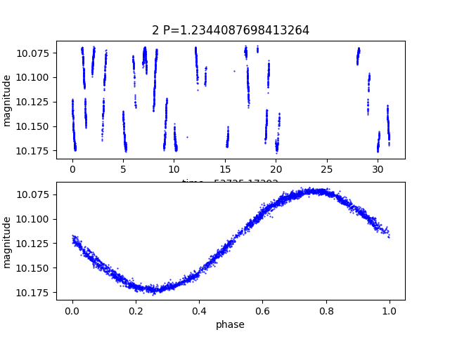
The plot below is the actual EXAMPLES/2.png produced by plotlc() — LC vs time on the top panel, phase-folded at the LS period on the bottom:
Example 4. Same as Example 3, but use process_all_lcs=True so the whole list goes through one -python call. With process_all_lcs enabled, vector inputs (t, ph, mag) arrive as lists of numpy arrays; scalar inputs (Name, LS_Period_1_0) arrive as numpy arrays of length Nlc, so the user code loops over each light curve manually.
code = (
    "for i in range(0, len(mag)):\n"
    "    plotlc(Name[i], 'EXAMPLES/', t[i], ph[i], mag[i], LS_Period_1_0[i])\n"
)
batch = (vt.Pipeline()
         .LS(0.1, 100., 0.1, npeaks=1)
         .Phase("ls", phasevar="ph")
         .python(code,
                 init="EXAMPLES/plotlc.py", init_fromfile=True,
                 process_all_lcs=True)
         ).run_filelist("EXAMPLES/lc_list",
                        perpoint_columns={"t": 1, "mag": 2, "err": 3})
Example 5. Reuse Python state across two -python calls in the same pipeline using continueprocess. The first call defines a module-global cached value; the second reads it. To survive across calls (which run inside per-call wrapper functions), mutable state must be declared global.
batch = (vt.Pipeline()
         .python("global _shared_mult\n_shared_mult = 1000.0",
                 invars="mag", outvars="mag")
         .python("global _shared_mult\n"
                 "b = _shared_mult * float(numpy.var(mag))",
                 continueprocess=1,
                 invars="mag", outvars="b", outputcolumns="b")
         ).run_filelist("EXAMPLES/lc_list",
                        perpoint_columns={"t": 1, "mag": 2, "err": 3})
print(batch.vars[["Name", "PYTHON_b_1"]])
Example 6. In-process mode (inprocess=True). User code shares the calling script's globals — it can reference imports, helpers, or class instances defined at module scope without going through init. This works only with single-LC Pipeline.run(lc) in library mode; batch entry points raise RuntimeError.
import numpy as np

# A helper defined in *your* script — visible to the -python body
# below because the in-process callback execs into __main__.__dict__.
def fancy_metric(arr):
    return float(np.std(arr) - np.median(np.diff(arr)))

lc = vt.LightCurve.from_file("EXAMPLES/2")
result = (vt.Pipeline()
          .python("b = fancy_metric(mag)",
                  invars="mag", outvars="b", outputcolumns="b",
                  inprocess=True)
          ).run(lc)
print(result.vars["PYTHON_b_0"])
To sandbox the inline code (so it can't see __main__), pass namespace=...:
sandbox = {"my_factor": 7.0}
lc = vt.LightCurve.from_file("EXAMPLES/2")
result = (vt.Pipeline()
          .python("b = my_factor * float(numpy.var(mag))",
                  invars="mag", outvars="b", outputcolumns="b",
                  inprocess=True, namespace=sandbox)
          ).run(lc)
print(result.vars["PYTHON_b_0"])