Extension Commands
pyvartools ships typed wrappers for the USERLIB extensions bundled with vartools and a generic integration layer for hand-written extensions.
User Extension Commands
vartools supports user-developed commands compiled as shared libraries (.so / .la). Eight such extensions are bundled with the source tree under USERLIBS/src/ — -fastchi2, -ftuneven, -hatpiflag, -jktebop, -macula, -magadd, -splinedetrend, and -stitch (see Extension Commands for the CLI reference). pyvartools ships typed Python wrappers for all eight, so they can be used exactly like a built-in command; it also exposes a generic integration layer for user-written extensions.
How extensions are loaded
If the library has been installed into the vartools userlibs data directory (e.g. via make install in USERLIBS/src/), vartools loads it automatically and no -L flag is needed:
If you want to load an extension that is not installed (or one that lives outside the installed search directory), pass it with -L path/to/lib.so placed immediately before the command flag. pyvartools mirrors both behaviours.
Bundled typed wrappers
Every bundled extension has a dedicated class in pyvartools.commands with typed parameters. Each constructor takes an optional lib_path= argument; omit it when the extension is installed and auto-loaded, or pass the path to the .so / .la file explicitly:
import pyvartools as vt
from pyvartools.commands import fastchi2, stitch

r = vt.fastchi2("EXAMPLES/2", Nharm=2, freqmax=24.0, freqmin=0.1)
Explicit lib_path= is supported for libraries that are not installed in the
default vartools userlibs directory; the path below is just an illustrative
placeholder:
...                                          # illustrative only
pipe = (vt.Pipeline()
        .fastchi2(Nharm=2, freqmax=24.0, freqmin=0.1,
             lib_path="/path/to/fastchi2.so"))
All typed-wrapper pipelines automatically run in subprocess mode (library/in-process mode does not support dynamically loaded extensions).
magadd — add a constant to magnitudes
Syntax
Description
Add a scalar offset to every magnitude in the light curve. The offset can be a fixed constant, a per-LC value from the input list, a previously computed output statistic, or an analytic expression. This is also the canonical template extension included in the source tree to demonstrate how to write user-defined VARTOOLS extensions.
CLI equivalent: -magadd.
Parameters
| Parameter | Type | Description |
|---|---|---|
value |
float or str |
Bare number → fix value; string → split as "fix v", "list [column N]", "fixcolumn NAME", or "expr EXPR". |
lib_path |
str, optional |
Path to magadd.so / magadd.la. Omit when installed and auto-loaded. |
Output
Suffix N is the pipeline command index:
| Column | Description |
|---|---|
Magadd_addval_N |
The offset value applied for that LC. |
Examples
from pyvartools.commands import magadd
pipe = vt.Pipeline().magadd(5.0)                      # fix 5.0
pipe = vt.Pipeline().magadd("fixcolumn MeanMag_0")    # from prior stats column
# Add 0.5 mag to every observation of EXAMPLES/2; the two rms calls show the
# mean magnitude shifts by 0.5 while the RMS is unchanged.
lc = vt.LightCurve.from_file("EXAMPLES/2")
result = (vt.Pipeline()
          .rms()
          .magadd(0.5)
          .rms()).run(lc)
print(result.vars["RMS_0"], result.vars["RMS_2"])
hatpiflag — HATPI binary flag combiner
Syntax
cmd.hatpiflag(fiphot_string_flag_var, rejbadframe_mask_var,
              tfa_outlier_mask_var, pointing_outlier_flag_var,
              output_flag_var, lib_path=None)
Description
Combine four per-observation HATPI quality indicators (fiphot string flag, reject-bad-frame mask, TFA-outlier mask, pointing-outlier flag) into a single bit-packed flag variable suitable for HATPI photometry pipelines. Each input contributes a different bit to the output:
- bits 0–3 (values 1, 2, 4, 8): set from the fiphot string flag —
X(bad photometry) sets bit 0,C(saturated/hot) sets bit 1,A(asteroid) sets bit 2,S(satellite) sets bit 3 (H/I/J/Kset combinations of bits 1–3). - bit 4 (value 16): set when the bad-frame mask flags the point as rejected.
- bit 5 (value 32): set when the TFA-outlier mask flags the point as an outlier.
- bit 6 (value 64): set when the pointing-outlier flag is 1.
CLI equivalent: -hatpiflag.
Parameters
| Parameter | Type | Description |
|---|---|---|
fiphot_string_flag_var |
str |
Name of the LC vector of one-character string flags from fiphot. |
rejbadframe_mask_var |
str |
Bad-frame mask vector (0 = rejected, 1 = keep). |
tfa_outlier_mask_var |
str |
TFA outlier mask vector (0 = outlier, 1 = keep). |
pointing_outlier_flag_var |
str |
Pointing outlier flag vector (1 = outlier, 0 = ok). |
output_flag_var |
str |
Name of the LC vector to receive the combined binary flag. |
lib_path |
str, optional |
Path to hatpiflag.so / hatpiflag.la. |
Output
hatpiflag writes its result into the named output LC vector (output_flag_var); it does not produce summary statistics directly. Use a downstream stats call to summarise the flag.
Examples
from pyvartools.commands import hatpiflag
pipe = (vt.Pipeline()
        .hatpiflag("fiphot_flag", "rejbadframe_mask",
              "tfa_outlier_mask", "pointing_outlier_flag", "quality_flag"))
# Read a 7-column LC (t/mag/err + four HATPI flag columns) and combine the
# four flag vectors into a single quality_flag.  The string-typed fiphot
# flag column is declared with vt.PerPointColumn(col=4, type="string") in the
# `perpoint_columns=` mapping.
batch = (vt.Pipeline()
         .hatpiflag("fiphot_flag", "rejbadframe", "tfa_mask",
                    "pointing_outlier", "quality_flag")
         .stats("quality_flag", "mean,sum,max")
         ).run_filelist(["EXAMPLES/2.hatpiflag"],
                        perpoint_columns={
                            "t": 1, "mag": 2, "err": 3,
                            "fiphot_flag": vt.PerPointColumn(col=4, type="string"),
                            "rejbadframe": 5,
                            "tfa_mask": 6,
                            "pointing_outlier": 7,
                        })
fastchi2 — Palmer (2009) fast chi² periodogram
Syntax
cmd.fastchi2(Nharm, freqmax, freqmin=None, detrendorder=None,
             t0=None, timespan=None, oversample=None, chimargin=None,
             Npeak=None, norefitpeak=False,
             save_per=False, save_model=False,
             omodelvariable=None, lib_path=None)
Description
Compute the Fast χ² periodogram using Palmer's algorithm, which searches for the best-fitting multi-harmonic sinusoidal model at each trial frequency. Each parameter accepts one of three sources: a number (emitted as fix N), or a string "fix V" / "list [column N]" / "fixcolumn NAME" / "expr EXPR".
CLI equivalent: -fastchi2.
Parameters
| Parameter | Type | Description |
|---|---|---|
Nharm |
value-spec | Number of harmonics in the model (1 = fundamental only, 2 = +first overtone, …). |
freqmax |
value-spec | Maximum search frequency (cycles/day). |
freqmin |
value-spec, optional | Minimum search frequency (default 0). |
detrendorder |
value-spec, optional | Polynomial order for pre-detrending (default 0). |
t0 |
value-spec, optional | Reference epoch for detrending. |
timespan |
value-spec, optional | Total time span used for the Nyquist frequency. |
oversample |
value-spec, optional | Oversampling factor for the periodogram grid. |
chimargin |
value-spec, optional | χ² margin for selecting periodogram peaks to refine. |
Npeak |
int, optional | Number of peaks to report. |
norefitpeak |
bool | Skip the fine peak search; emit raw periodogram peaks only. |
save_per |
bool, str, or Output |
Periodogram output file. True captures as result.files["fastchi2_per_N"]. |
save_model |
bool, str, or Output |
Best-fit harmonic model output file. |
omodelvariable |
str, optional |
Name of an LC vector to store the model curve. |
lib_path |
str, optional |
Path to fastchi2.so / fastchi2.la. |
Output
Per peak k (1 to Npeak) and command index N:
| Column | Description |
|---|---|
Fastchi2_Frequency_k_N |
Frequency (cycles/day) of peak k. |
Fastchi2_Chi2Reduction_k_N |
χ² reduction at the peak (χ²₀ − χ² of the harmonic fit). |
When the corresponding save_* keyword is set:
| File key | Description |
|---|---|
result.files["fastchi2_per_N"] |
DataFrame: frequency vs. χ² periodogram. |
result.files["fastchi2_model_N"] |
DataFrame: best-fit harmonic model evaluated at the observed times. |
References
Cite Palmer 2009, ApJ, 695, 496.
Examples
from pyvartools.commands import fastchi2
pipe = (vt.Pipeline()
        .fastchi2(Nharm=2, freqmax=24.0, freqmin=0.1,
             oversample=4, Npeak=3, save_per=True))
# Run Palmer's Fast chi^2 periodogram on EXAMPLES/2; search 0.1–10 cyc/day
# with one harmonic and capture the periodogram.
lc = vt.LightCurve.from_file("EXAMPLES/2")
result = lc.fastchi2(Nharm=1, freqmax=10.0, freqmin=0.1,
                     save_per="EXAMPLES/OUTDIR1")
splinedetrend — basis-spline / poly / harmonic detrending
Syntax
cmd.splinedetrend(detrendvecs, sigmaclip=None,
                  save_model=False, save_coeffs=False,
                  omodelvariable=None, lib_path=None)
Description
Fit a multivariate linear model to the light-curve magnitudes against one or more auxiliary variables (e.g. time, CCD x/y position, CCD temperature). Cross-terms between variables are not included.
Three basis types are supported per detrending variable: spline:knotspacing:order (B-spline basis using GSL gsl_bspline_eval), poly:order (polynomial), and harm:nharm (harmonic series; nharm=0 for fundamental only with period = 2× variable range). Append :groupbygap:gapsize to split the fit at gaps in the variable larger than gapsize.
CLI equivalent: -splinedetrend.
Parameters
| Parameter | Type | Description |
|---|---|---|
detrendvecs |
str or list |
Single comma-joined string or a list of VAR:<spline:knotspacing:order \| poly:order \| harm:nharm>[:groupbygap:gapsize] specs. |
sigmaclip |
value-spec, optional | Sigma-clip threshold; outliers above this σ level are excluded from the fit (the model is still evaluated and subtracted at clipped points). |
save_model |
bool, str, or Output |
Best-fit model output file. True captures as result.files["splinedetrend_model_N"]. |
save_coeffs |
bool, str, or Output |
Linear basis coefficients output file. |
omodelvariable |
str, optional |
Comma-separated outvar[:inputvar] list specifying per-variable model contributions to store as LC vectors. |
lib_path |
str, optional |
Path to splinedetrend.so / splinedetrend.la. |
Output
Suffix N is the pipeline command index:
| Column | Description |
|---|---|
Splinedetrend_MedianMagnitude_N |
Median magnitude added back to the detrended LC. |
Splinedetrend_NOutliers_N |
Number of clipped outliers. |
Splinedetrend_NDataGroups_N |
Number of fit groups created by groupbygap. |
Splinedetrend_NFitParamsTotal_N |
Total free-parameter count of the model. |
When the corresponding save_* keyword is set:
| File key | Description |
|---|---|
result.files["splinedetrend_model_N"] |
Best-fit model evaluated at the observed times. |
result.files["splinedetrend_coeffs_N"] |
Linear basis coefficients. |
Examples
from pyvartools.commands import splinedetrend
pipe = (vt.Pipeline()
        .splinedetrend(["t:spline:0.1:3", "x:poly:2", "y:poly:2"],
                  sigmaclip=4.0, save_model=True))
The canonical example (a TESS sector-1 LC for GAIA DR2 6479535620075955328) reads several auxiliary columns (x, y, temp) from a FITS file. Because that requires a non-default -inputlcformat flag while loading the LC inside vartools, the cleanest Python equivalent invokes vartools directly via subprocess.
import subprocess
subprocess.run([
    "vartools",
    "-i", "EXAMPLES/6479535620075955328_llc.fits",
    "-inputlcformat", "t:TMID_BJD,mag:IRM1,err:IRE1,x:XIC,y:YIC,temp:CCDTEMP",
    "-expr", "magorig=mag",
    "-splinedetrend",
    "t:spline:1.0:3:groupbygap:0.5,x:poly:1,y:poly:1,temp:poly:1",
    "sigmaclip", "fix", "3.0",
    "omodel", "EXAMPLES/OUTDIR1/",
    "omodelcoeffs", "EXAMPLES/OUTDIR1/",
    "omodelvariable", "tmod:t,xmod:x,ymod:y,tempmod:temp",
    "-o", "EXAMPLES/OUTDIR1/6479535620075955328.splinedetrend.lc.txt",
    "columnformat", "t,magorig,mag,err,x,y,temp,tmod,xmod,ymod,tempmod",
    "-rms", "-oneline",
], check=True)
ftuneven — complex Fourier transform of unevenly-sampled data
Syntax
cmd.ftuneven(output_vectors=None, output_file=False,
             save_outdir=None, nameformat=None,
             freqauto=False, freqrange=None,
             freqvariable=None, freqfile=None,
             ft_sign=None, tt_zero=None,
             changeinputvectors=None, lib_path=None)
Description
Compute the complex Fourier transform of an unevenly sampled time series using Scargle's method. Returns the real and imaginary components plus the absolute-square power spectrum (equivalent to the Lomb-Scargle periodogram). Input and output frequencies are in radians per unit time.
At least one output mode (output_vectors, output_file, or both) and exactly one frequency source (freqauto, freqrange, freqvariable, or freqfile) must be specified. To write both LC vectors and a per-LC file, pass output_vectors=(...) together with output_file=True (or a path). freqrange is a (min, max, step) tuple of value-specs.
CLI equivalent: -ftuneven.
Parameters
Output mode (at least one; both may be combined):
| Parameter | Type | Description |
|---|---|---|
output_vectors |
tuple of 4 str, optional |
Names of LC vectors (freq, FTreal, FTimag, periodogram); all LC vectors are resized to the transform length. |
output_file |
bool, str, or Output, optional |
Write per-LC files (default name BASELC.ftuneven; four whitespace columns: freq, FT_real, FT_imag, periodogram). |
save_outdir |
str, optional |
Directory used when output_file=True; overrides the pipeline temp dir. |
nameformat |
str, optional |
Format string for the per-LC output filename. |
Frequency source (choose one):
| Parameter | Type | Description |
|---|---|---|
freqauto |
bool |
Determine frequencies automatically from the time baseline and cadence. |
freqrange |
(min, max, step) tuple of value-specs |
Uniform grid. |
freqvariable |
str |
Read frequencies from an existing LC vector. |
freqfile |
str |
Read frequencies from the first column of an ASCII file (used identically for every LC). |
| Parameter | Type | Description |
|---|---|---|
ft_sign |
int or str, optional |
Sign of the transform: −1 (default) = forward; +1 = inverse. |
tt_zero |
float or str, optional |
Time origin (default 0). |
changeinputvectors |
tuple of 3 str, optional |
Apply the transform to vectors other than t/mag: (tvec, data_real_vec, data_imag_vec). |
lib_path |
str, optional |
Path to ftuneven.so / ftuneven.la. |
Output
ftuneven writes its results into the named LC vectors and/or per-LC output files; it does not produce summary statistics directly.
References
Cite Scargle 1989, ApJ, 343, 874.
Examples
from pyvartools.commands import ftuneven

# Write the FT into four light-curve variables
pipe = (vt.Pipeline()
        .ftuneven(output_vectors=("freq", "ft_real", "ft_imag", "periodogram"),
             freqrange=(0.01, 10.0, 0.001)))

# Write the FT to a per-LC file using an automatic frequency grid
pipe = vt.Pipeline().ftuneven(output_file=True, freqauto=True)
# Compute Scargle's complex Fourier transform of EXAMPLES/2 over a uniform
# frequency grid (radians per unit time), writing the FT to a per-LC file.
lc = vt.LightCurve.from_file("EXAMPLES/2")
result = lc.ftuneven(output_file="EXAMPLES/OUTDIR1",
                     freqrange=(0.05, 5.0, 0.001))
stitch — stitch multi-segment light curves at offsets
Syntax
cmd.stitch(stitch_variables, uncertainty_variables, mask_variables,
           lcnum_var, method,
           refnum_var=None, groupbytime=None, groupbytime_start=None,
           fitonly=False, noshiftmasked=False, refmag=None,
           save_fitted_parameters=False, fitted_parameters_nameformat=None,
           add_stitchparams_fitsheader=False, add_stitchparams_mode=None,
           add_shifts_fitsheader=None, add_shifts_hdu=None,
           add_shifts_mode=None,
           shifts_file=None, append_refnum_to_fieldlabel=False,
           in_shifts_file=None, nobs_refit=None,
           header_basename_only=False,
           out_shifts_file=None, include_missing=False,
           lib_path=None)
Description
Designed for use with the -l "combinelcs" (or -i "combinelcs") input mode, -stitch fits for and removes additive offsets between distinct light-curve segments (e.g. observations from different telescopes, cameras, or fields).
method is one of "median", "mean", "weightedmean", "poly ORDER", or "harmseries PERIODVAR NHARM".
CLI equivalent: -stitch.
Parameters
| Parameter | Type | Description |
|---|---|---|
stitch_variables |
str or list of str |
Magnitude variable(s) to stitch (typically "mag"). |
uncertainty_variables |
str or list of str |
Uncertainties for each magnitude variable (typically "err"). |
mask_variables |
str or list of str |
Mask vector(s); points with mask = 0 (or negative) are excluded from the fit (> 0 = include). By default an excluded point still has the fitted per-segment shift applied to it — masking affects only the fit, not the correction (see noshiftmasked). |
lcnum_var |
str |
Variable identifying which input segment each observation belongs to (typically set by the lcnumvar keyword of combinelcs). |
method |
str, required |
"median", "mean", "weightedmean", "poly ORDER", or "harmseries PERIODVAR NHARM". |
refnum_var |
str, optional |
Further subdivide segments by a second grouping variable. |
groupbytime |
float, optional |
Group segments into time bins; the bin size is automatically widened if necessary so all segments can be inter-calibrated. |
groupbytime_start |
float, optional |
Start time of the first time bin (only meaningful when groupbytime is set). |
fitonly |
bool |
Compute the shifts but do not subtract them. |
noshiftmasked |
bool |
Leave masked points unshifted, so that masking excludes a point from both the fit and the correction. By default masked points are shifted along with their segment. |
refmag |
float or str, optional |
Shift all groups to a reference magnitude rather than adopting one group as the (unshifted) reference. A number is passed as fix value; a string is "fix V" / "list" / "fixcolumn COL" / "expr E", or a bare expression. For median/mean/weightedmean without groupbytime every group's statistic is shifted to the value; with groupbytime, or for poly/harmseries, the reference group's level (its median for poly/harmseries) is tied to it. The shifts (including the reference group's) are recorded so unstitch can undo them. |
save_fitted_parameters |
bool, str, or Output |
Write per-source shift files. |
fitted_parameters_nameformat |
str, optional |
Format string applied to the fitted-parameter filenames (format keyword). |
add_stitchparams_fitsheader |
bool or str |
Add stitch parameters to the FITS header. Pass True, or "primary"/"extension" to select the HDU. |
add_stitchparams_mode |
str, optional |
"append" or "update". |
add_shifts_fitsheader |
str, optional |
Keyword base (e.g. "SHFT") used to log shifts into FITS headers. |
add_shifts_hdu |
str, optional |
"primary" or "extension". |
add_shifts_mode |
str, optional |
"append" or "update". |
shifts_file |
tuple of 2 str, optional |
(fieldlabelsvar, starnamevar) — enables shifts_file mode for reading/writing previously determined shifts. |
append_refnum_to_fieldlabel |
bool |
Append the refnum_var value to the field label in shifts files. |
in_shifts_file |
str or list of str, optional |
Pre-existing shifts file(s) to read. One file per stitched variable — pass a single string when stitch_variables is a string, or a list of the same length as stitch_variables when it is a list. |
nobs_refit |
int, optional |
Minimum new observations before re-fitting an existing shift. |
header_basename_only |
bool |
Match shifts-file rows by basename only. |
out_shifts_file |
str or list of str, optional |
Output shifts file(s) to write. One file per stitched variable — pass a single string when stitch_variables is a string, or a list of the same length as stitch_variables when it is a list. |
include_missing |
bool |
Include un-fit (missing) sources in the output shifts file. |
lib_path |
str, optional |
Path to stitch.so / stitch.la. |
Output
Suffix N is the pipeline command index:
| Column | Description |
|---|---|
Stitch_NLCGroups_N |
Number of LC segment groups. |
Stitch_NTimeGroups_N |
Number of time-bin groups. |
Stitch_NFitParamsTotal_N |
Total free-parameter count of the stitch fit. |
When save_fitted_parameters is set:
| File key | Description |
|---|---|
result.files["stitch_fitted_parameters_N"] |
Per-source shift file (suffix .stitch). |
Examples
from pyvartools.commands import stitch
pipe = (vt.Pipeline()
        .stitch("mag", "err", "mask", "lcnum", method="median",
           groupbytime=30.0, save_fitted_parameters=True))

# Multiple magnitude/uncertainty/mask variables
pipe = (vt.Pipeline()
        .stitch(["mag_ap1", "mag_ap2"], ["err_ap1", "err_ap2"],
           ["mask_ap1", "mask_ap2"], "lcnum", method="poly 3"))
-stitch is most useful with the -l ... combinelcs input mode, which combines multiple files into a single in-memory LC. The cleanest way to drive that from pyvartools is Pipeline.run_combinelc() for a single combined LC or run_combinelcs() for many groups; both default to emitting lcnumvar lcnum, which -stitch consumes.
import pyvartools as vt
from pyvartools.commands import stitch

# Combine EXAMPLES/2 and EXAMPLES/2.shifted (= EXAMPLES/2 with +0.3 mag) into a
# single LC and remove the inter-segment offset by median.  The two -rms calls
# show the offset before and after stitching.
result = (vt.Pipeline()
          .expr("mask=mag*0+1")
          .rms()
          .stitch("mag", "err", "mask", "lcnum", method="median")
          .rms()
          ).run_combinelc(["EXAMPLES/2", "EXAMPLES/2.shifted"])
print(result.vars[["RMS_1", "RMS_3"]])   # before / after stitching
With refmag the segments are shifted onto a common reference magnitude rather than onto one reference segment. For the median method (no groupbytime) every segment's median lands on the value, so the combined median does too:
import pyvartools as vt

result = (vt.Pipeline()
          .expr("mask=mag*0+1")
          .stitch("mag", "err", "mask", "lcnum", method="median", refmag=12.0)
          .stats("mag", "median")
          ).run_combinelc(["EXAMPLES/2", "EXAMPLES/2.shifted"])
medkey = [k for k in result.vars.index if "MEDIAN" in k][0]
print(result.vars[medkey])   # ~ 12.0
Per-segment field labels and per-LC star names with shifts_file
shifts_file=(fieldlabelsvar, starnamevar) enables shifts-file mode, which writes (and optionally reads) measured offsets keyed by a per-observation field label and per-LC star name. The two values play different roles: fieldlabelsvar is a per-segment label (one value for each input file in the combined LC) and starnamevar is a single value for the combined LC as a whole. Supply them through the matching perlcsegment_vars and perlc_vars keywords on run_combinelc() / run_combinelcs():
import pyvartools as vt

# EXAMPLES/2.shifted is EXAMPLES/2 with +0.3 mag added.  Tag the two
# segments "2_A" / "2_B" so the recovered shifts file can attribute the
# 0.3 mag offset to segment B; tag the combined LC with starname "2".
result = (vt.Pipeline()
          .expr("mask=1")
          .stitch("mag", "err", "mask", "lcnum",
                  method="poly 5", groupbytime=0.5,
                  groupbytime_start=54550.123, fitonly=True,
                  shifts_file=("fieldname", "starname"),
                  out_shifts_file="/tmp/shifts.txt")
          ).run_combinelc(
              ["EXAMPLES/2", "EXAMPLES/2.shifted"],
              perlcsegment_vars={"fieldname": ["2_A", "2_B"]},
              perlc_vars={"starname": "2"},
          )
print(open("/tmp/shifts.txt").read())
# 2 2_A,0,3313;2_B,0.30000000000003313,3313
The first column of the output shifts file is the star name; the second is a ;-separated list of <field>,<shift>,<nobs> triplets. See run_combinelcs() for the full specification of perlcsegment_vars / perlc_vars, including how to pass a (values, type) tuple to override the auto-detected type.
unstitch — undo a stitch
Syntax
cmd.unstitch(unstitch_variables, source,
             fieldlabelsvar=None, starnamevar=None, in_shifts_file=None,
             append_refnum_to_fieldlabel=None,
             keywordbase=None, lcnum_var=None, refnum_var=None, hdu=None,
             maskpoints=None, noshiftmasked=False,
             strip_fitsheader=None, strip_stitchparams=False, strip_hdu=None,
             lib_path=None)
Description
The inverse of stitch: it adds the per-segment shifts that -stitch determined back to the light curve, recovering the pre-stitch magnitudes. The shifts come either from a file written by stitch's out_shifts_file (source="in_shifts_file") or from the keywords stitch's add_shifts_fitsheader wrote into the input FITS header (source="fitsheader").
CLI equivalent: -unstitch.
Parameters
| Parameter | Type | Description |
|---|---|---|
unstitch_variables |
str or list of str |
Magnitude variable(s) to un-shift (typically "mag"). For the "in_shifts_file" source, one input shifts file per variable, in the same order. |
source |
str, required |
"in_shifts_file" or "fitsheader". |
fieldlabelsvar |
str |
(in_shifts_file) Per-point string field identifier used to match points to shifts. Required for this source. |
starnamevar |
str |
(in_shifts_file) Per-LC string star name selecting the file row. Required for this source. |
in_shifts_file |
str or list of str |
(in_shifts_file) Shifts file(s), one per variable. Required for this source. |
append_refnum_to_fieldlabel |
str, optional |
(in_shifts_file) Refnum variable, if the file's labels had the refnum appended. |
keywordbase |
str |
(fitsheader) Keyword basename stitch used (e.g. "SHFT"). Required for this source. |
lcnum_var |
str |
(fitsheader) Variable identifying the segment for each point. Required for this source. |
refnum_var |
str, optional |
(fitsheader) Refnum variable, if the shifts used one. |
hdu |
str, optional |
(fitsheader) "primary" (default) or "extension" — which header to read. |
maskpoints |
str, optional |
Mask variable. Masked points are exempt from the coverage check; by default a masked point that matches a shift is still un-shifted (see noshiftmasked). |
noshiftmasked |
bool |
Leave masked points completely unchanged. Requires maskpoints. Use to invert a stitch run that used its own noshiftmasked. |
strip_fitsheader |
str, optional |
Keyword basename to remove from the output FITS header (e.g. with -o ... fits copyheader). |
strip_stitchparams |
bool |
Also remove the fixed STCH* stitch-parameter keywords. |
strip_hdu |
str, optional |
"primary" (default) or "extension" — which header to strip. |
lib_path |
str, optional |
Path to unstitch.so / unstitch.la. |
Constructor-time validation enforces the source-specific required parameters, that noshiftmasked is given only with maskpoints, and that hdu / strip_hdu are "primary" or "extension".
Output
Suffix N is the pipeline command index:
| Column | Description |
|---|---|
Unstitch_Npoints_shifted_N |
Number of points that received a shift. |
-unstitch requires every unmasked point to be covered by the supplied shifts; if not, the run raises RunError (the wrong shifts are being used).
Examples
Re-stitch EXAMPLES/2 + EXAMPLES/2.shifted and immediately undo it, reading the shifts from the file shipped in EXAMPLES/OUTDIR1 (written by an earlier stitch run with out_shifts_file). The per-segment field labels fA/fB and star name star1 are supplied through perlcsegment_vars / perlc_vars, matching the labels in that file. The three RMS columns show the scatter inflated by the offset, dropping after stitching, and returning after un-stitching.
import pyvartools as vt

result = (vt.Pipeline()
          .expr("mask=mag*0+1")
          .rms()
          .stitch("mag", "err", "mask", "lcnum", method="median")
          .rms()
          .unstitch("mag", source="in_shifts_file",
                    fieldlabelsvar="field", starnamevar="star",
                    in_shifts_file="EXAMPLES/OUTDIR1/shifts.txt")
          .rms()
          ).run_combinelc(["EXAMPLES/2", "EXAMPLES/2.shifted"],
                          perlcsegment_vars={"field": ["fA", "fB"]},
                          perlc_vars={"star": "star1"})
print(result.vars[["RMS_1", "RMS_3", "RMS_5"]])   # inflated / stitched / restored
For the "fitsheader" source — recovering the shifts from FITS-header keywords written by stitch add_shifts_fitsheader, and optionally removing them again with strip_fitsheader — see the CLI example.
jktebop — detached eclipsing-binary model
Syntax
cmd.jktebop(mode,
            Period=None, vary_Period=False,
            T0=None, vary_T0=False,
            r1_r2=None, vary_r1_r2=False,
            r2_r1=None, vary_r2_r1=False,
            M2_M1=None, vary_M2_M1=False,
            J2_J1=None, vary_J2_J1=False,
            i=None, vary_i=False,
            bimpact=None, vary_bimpact=False,
            esinomega=None, vary_esinomega=False,
            ecosomega=None, vary_ecosomega=False,
            LD1_law="quad", LD1_coeffs=(0.3, 0.3), vary_LD1=False,
            LD2_law="lockLD1", LD2_coeffs=(), vary_LD2=False,
            gravdark1=None, vary_gravdark1=False,
            gravdark2=None, vary_gravdark2=False,
            reflection1=None, vary_reflection1=False,
            reflection2=None, vary_reflection2=False,
            L3=None, vary_L3=False,
            tidallag=None, vary_tidallag=False,
            correctlc=False,
            save_model=False, model_nameformat=None,
            save_curve=False, curve_xaxis=None,
            curve_step=None, curve_nameformat=None,
            lib_path=None)
Description
Fit or inject a JKTEBOP detached eclipsing-binary light-curve model. Use mode="inject" to add the model to the light curve, or mode="fit" to optimise the parameters. Pass vary_*=True to free the corresponding parameter during fitting.
Every mandatory parameter (Period, T0, r1_r2, r2_r1, M2_M1, J2_J1, i or bimpact, esinomega, ecosomega) is a value-spec; the corresponding vary_*=True flag frees that parameter in the fit. Optional physical parameters: gravdark1/2 (default 1.0), reflection1/2 (computed if absent or ≤ 0), L3 (third light, default 0), tidallag (default 0). Limb-darkening laws are "linear", "quad", "log", "sqrt"; LD2_law="lockLD1" forces the secondary to share the primary's coefficients.
CLI equivalent: -jktebop.
Parameters
| Parameter | Type | Description |
|---|---|---|
mode |
str |
"inject" or "fit". |
Period |
value-spec | Orbital period in days. |
T0 |
value-spec | Central time of a primary eclipse. |
r1_r2 |
value-spec | Sum of stellar radii divided by the semi-major axis (r1+r2). |
r2_r1 |
value-spec | Ratio of stellar radii (r2/r1). |
M2_M1 |
value-spec | Mass ratio. |
J2_J1 |
value-spec | Surface brightness ratio. |
i |
value-spec, optional | Orbital inclination in degrees (90° = edge-on). |
bimpact |
value-spec, optional | Impact parameter at primary eclipse (alternative to i; 0 = central, 1 = grazing). |
esinomega, ecosomega |
value-spec | e sin ω and e cos ω. |
LD1_law |
str |
"linear", "quad", "log", or "sqrt". |
LD1_coeffs |
tuple of 1 or 2 floats/strings | Limb-darkening coefficients. |
LD2_law |
str |
"lockLD1", "linear", "quad", "log", or "sqrt". |
LD2_coeffs |
tuple, optional | Used only when LD2_law is not "lockLD1". |
gravdark1, gravdark2 |
value-spec, optional | Gravity-darkening coefficients (default 1.0). |
reflection1, reflection2 |
value-spec, optional | Reflection coefficients (computed if absent). |
L3 |
value-spec, optional | Third light (default 0). |
tidallag |
value-spec, optional | Tidal lag in degrees (default 0). |
vary_* |
bool |
Free the corresponding parameter during fitting. |
correctlc |
bool |
Subtract the best-fit model from the LC. |
save_model |
bool, str, or Output |
Write the model evaluated at the observed times. |
model_nameformat |
str, optional |
Format string for the saved model filename. |
save_curve |
bool, str, or Output |
Write a uniformly sampled model curve. |
curve_xaxis |
"jd" or "phase", optional |
Axis for the saved curve. |
curve_step |
float, optional |
Step size for the saved curve. |
curve_nameformat |
str, optional |
Format string for the saved curve filename. |
lib_path |
str, optional |
Path to jktebop.so / jktebop.la. |
Output
Suffix N is the pipeline command index. The base parameter columns are produced unconditionally:
| Column | Description |
|---|---|
Jktebop_PERIOD_N |
Best-fit (or injected) orbital period. |
Jktebop_T0_N |
Best-fit (or injected) reference epoch. |
Jktebop_R1+R2_N |
Best-fit (or injected) sum of fractional radii. |
Jktebop_R2/R1_N |
Best-fit (or injected) ratio of radii. |
Jktebop_M2/M1_N |
Best-fit (or injected) mass ratio. |
Jktebop_J2/J1_N |
Best-fit (or injected) surface-brightness ratio. |
Jktebop_INCLINATION_N |
Inclination (degrees). |
Jktebop_bimpact_N |
Impact parameter at primary eclipse. |
Jktebop_ESINOMEGA_N |
e sin ω. |
Jktebop_ECOSOMEGA_N |
e cos ω. |
Jktebop_STAR1_LD_COEFF_1_N |
Primary limb-darkening coefficient #1. |
Jktebop_STAR1_LD_COEFF_2_N |
Primary limb-darkening coefficient #2 (if the law has two). |
Conditional columns (added only when the input is set):
| Column | Condition |
|---|---|
Jktebop_STAR2_LD_COEFF_1_N, Jktebop_STAR2_LD_COEFF_2_N |
When LD2_law is not "lockLD1". |
Jktebop_GRAVDARK1_N, Jktebop_GRAVDARK2_N |
When gravdark1 / gravdark2 is given. |
Jktebop_REFLECTION1_N, Jktebop_REFLECTION2_N |
When reflection1 / reflection2 is given. |
Jktebop_L3_N |
When L3 is given. |
Jktebop_TIDALLAG_N |
When tidallag is given. |
Jktebop_CHI2_N, Jktebop_NDOF_N |
When mode="fit" (best-fit χ² and degrees of freedom). |
When save_model is set, vartools writes a per-LC ASCII file with the columns Time Mag_lc Err Mag_model. The file suffix is .jktebop.
When save_curve is set, vartools writes a uniformly-sampled model curve. With curve_xaxis="phase" (default "jd") the file has columns #Phase Mag_model; with curve_xaxis="jd" it has #Time Mag_model Phase. The step size is curve_step (default 0.01 days for JD mode, 0.01 in fractional phase for phase mode). The file suffix is .jktebopcurve and the captured key is result.files["jktebop_curve_N"].
References
Cite Southworth et al. 2004, MNRAS, 351, 1277; Popper & Etzel 1981, AJ, 86, 102; Etzel 1981, Photometric and Spectroscopic Binary Systems, 111; Nelson & Davis 1972, ApJ, 174, 617.
Examples
from pyvartools.commands import jktebop
pipe = (vt.Pipeline()
        .jktebop("fit",
            Period=2.5,     vary_Period=True,
            T0=0.0,         vary_T0=True,
            r1_r2=0.3, r2_r1=0.5, M2_M1=1.0, J2_J1=1.0,
            i=89.0,         vary_i=True,
            esinomega=0.0, ecosomega=0.0,
            LD1_law="quad", LD1_coeffs=(0.3, 0.3),
            LD2_law="lockLD1",
            correctlc=True, save_model=True))
# Inject a JKTEBOP detached EB signal (P=2.5d, R2/R1=0.5, J2/J1=0.3, i=89 deg,
# circular orbit, quadratic LD) into EXAMPLES/3 and recover the primary eclipse
# with -BLS.
lc = vt.LightCurve.from_file("EXAMPLES/3")
result = (vt.Pipeline()
          .jktebop("inject",
                   Period=2.5, T0=53727.0,
                   r1_r2=0.15, r2_r1=0.5,
                   M2_M1=0.6, J2_J1=0.3,
                   i=89.0,
                   esinomega=0.0, ecosomega=0.0,
                   LD1_law="quad", LD1_coeffs=(0.3, 0.3),
                   LD2_law="lockLD1",
                   save_model="EXAMPLES/OUTDIR1/")
          .BLS(1.0, 5.0, rmin=0.01, rmax=0.1,
               nbins=200, nfreq=5000, npeaks=1)).run(lc)
# Capture the uniformly-sampled phase-folded model curve (one row per
# 0.01-phase step) into result.files["jktebop_curve_0"].
lc = vt.LightCurve.from_file("EXAMPLES/3")
r = (vt.Pipeline()
     .jktebop("inject",
              Period=2.5, T0=53727.0,
              r1_r2=0.15, r2_r1=0.5, M2_M1=0.6, J2_J1=0.3,
              i=89.0,
              esinomega=0.0, ecosomega=0.0,
              LD1_law="quad", LD1_coeffs=(0.3, 0.3),
              LD2_law="lockLD1",
              save_curve=True, curve_xaxis="phase", curve_step=0.01)
     ).run(lc)
curve = r.files["jktebop_curve_0"]   # 2 columns: phase, model magnitude
print(curve.shape, curve.head(3))
macula — Kipping (2012) spot model
Syntax
cmd.macula(mode, *,
           Prot=None, vary_Prot=False,
           istar=None, vary_istar=False,
           kappa2=None, vary_kappa2=False,
           kappa4=None, vary_kappa4=False,
           c1=None, vary_c1=False, c2=None, vary_c2=False,
           c3=None, vary_c3=False, c4=None, vary_c4=False,
           d1=None, vary_d1=False, d2=None, vary_d2=False,
           d3=None, vary_d3=False, d4=None, vary_d4=False,
           blend=None, vary_blend=False,
           spots=None,
           fluxinput=False, fluxoutput=False, correctlc=False,
           save_model=False, model_tdelv=False, model_nameformat=None,
           save_curve=False, curve_tdelv=False,
           curve_step=None, curve_nameformat=None,
           lib_path=None)
Description
Fit or inject Kipping's Macula analytic model for starspot modulation. Use mode="inject" to add the model signal to the light curve, or mode="fit amoeba" (Nelder-Mead simplex) / mode="fit lm" (Levenberg-Marquardt) to optimise the parameters. Pass vary_*=True to mark a global parameter free during fitting.
Each of the 13 global parameters (Prot, istar, kappa2, kappa4, c1–c4, d1–d4, blend) is a keyword-argument value-spec with a matching vary_<name> flag. spots is a list of dicts, one per active spot, each providing value-specs for the eight per-spot parameters (Lambda0, Phi0, alphamax, fspot, tmax, life, ingress, egress). Individual spot parameters can be marked free by passing a (value, True) tuple (or a "vary_<name>": True entry in the dict).
CLI equivalent: -macula.
Parameters
Stellar parameters:
| Parameter | Type | Description |
|---|---|---|
mode |
str |
"inject", "fit amoeba", or "fit lm". |
Prot |
value-spec | Equatorial rotation period (LC time units). |
istar |
value-spec | Stellar inclination (radians). |
kappa2, kappa4 |
value-spec | Quadratic / quartic differential-rotation coefficients. |
c1–c4 |
value-spec | Stellar limb-darkening coefficients. |
d1–d4 |
value-spec | Spot limb-darkening coefficients. |
blend |
value-spec | Blend parameter. |
Per-spot dict keys (one entry in spots per active spot):
| Key | Description |
|---|---|
Lambda0 |
Longitude at maximum spot size (radians). |
Phi0 |
Latitude at maximum spot size (radians). |
alphamax |
Maximum angular radius (radians). |
fspot |
Spot-to-star flux contrast. |
tmax |
Reference epoch of maximum spot size. |
life |
Spot lifetime, FWHM (LC time units). |
ingress |
Spot growth duration. |
egress |
Spot decay duration. |
Output / control flags:
| Parameter | Type | Description |
|---|---|---|
vary_<name> |
bool |
Free the corresponding global parameter during fitting. |
fluxinput, fluxoutput |
bool |
Toggle flux vs. magnitude input/output (default: magnitudes). |
correctlc |
bool |
Subtract the model from the LC. |
save_model |
bool, str, or Output |
Write the model evaluated at the observed times (suffix .macula). |
model_tdelv |
bool |
Include predicted transit-depth variations in the saved model. |
model_nameformat |
str, optional |
Format string for the model filename. |
save_curve |
bool, str, or Output |
Write the model on a uniformly sampled time grid (suffix .maculacurve). |
curve_tdelv |
bool |
Include predicted transit-depth variations in the saved curve. |
curve_step |
float, optional |
Grid spacing for the saved curve. |
curve_nameformat |
str, optional |
Format string for the curve filename. |
lib_path |
str, optional |
Path to macula.so / macula.la. |
Output
Suffix N is the pipeline command index, and s is the 0-indexed spot number.
Always-emitted columns (one per global parameter and per per-spot parameter):
| Column | Description |
|---|---|
Macula_Prot_N |
Equatorial rotation period. |
Macula_Istar_N |
Stellar inclination (radians). |
Macula_kappa2_N, Macula_kappa4_N |
Differential-rotation coefficients. |
Macula_c1_N–Macula_c4_N |
Stellar limb-darkening coefficients. |
Macula_d1_N–Macula_d4_N |
Spot limb-darkening coefficients. |
Macula_blend_N |
Blend parameter. |
Macula_lambda0_s_N |
Spot s longitude at max size. |
Macula_phi0_s_N |
Spot s latitude at max size. |
Macula_alphamax_s_N |
Spot s maximum angular radius. |
Macula_fspot_s_N |
Spot s flux contrast. |
Macula_tmax_s_N |
Spot s reference epoch. |
Macula_life_s_N |
Spot s lifetime FWHM. |
Macula_ingress_s_N, Macula_egress_s_N |
Spot s ingress/egress durations. |
Fit-mode columns (added when mode starts with "fit"):
| Column | Description |
|---|---|
Macula_CHI2_N |
Best-fit χ². |
Macula_NDOF_N |
Degrees of freedom. |
The values reported in the parameter columns are the best-fit values when the matching vary_* is true, otherwise the input value (or, in "inject" mode, the value injected). Macula does not emit separate uncertainty columns.
When the corresponding save_* keyword is set:
| File key | Description |
|---|---|
result.files["macula_model_N"] |
Model evaluated at the observed times. |
result.files["macula_curve_N"] |
Uniformly sampled model curve. |
References
Cite Kipping 2012, MNRAS, 427, 2487.
Examples
from pyvartools.commands import macula
pipe = (vt.Pipeline()
        .macula("fit lm",
           Prot=10.0, vary_Prot=True,
           istar=1.4, kappa2=0.0, kappa4=0.0,
           c1=0.2, c2=0.1, c3=0.0, c4=0.0,
           d1=0.2, d2=0.1, d3=0.0, d4=0.0,
           blend=1.0,
           spots=[{
               "Lambda0": 0.0, "Phi0": 1.23, "alphamax": 0.2,
               "fspot": 0.1, "tmax": 0.0, "life": 1000.0,
               "ingress": 0.1, "egress": 0.1,
           }],
           save_model=True))
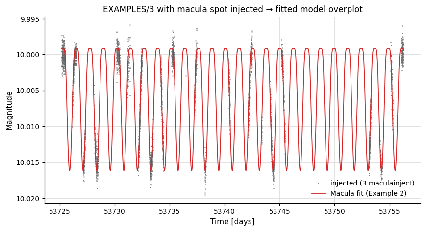
# Inject a single spotted-star light curve into EXAMPLES/3 (Macula's
# "inject" mode), using the LC time sampling and replacing the magnitudes
# with Gaussian noise.  tmax is set to the start time computed by `stats`.
lc = vt.LightCurve.from_file("EXAMPLES/3")
pipe = (vt.Pipeline()
        .stats("t", "min")
        .expr("mag=10.0+err*gauss()")
        .macula(
            "inject",
            Prot=1.234567, istar=1.4567,
            kappa2=0.0, kappa4=0.0,
            c1=0.2, c2=0.1, c3=0.0, c4=0.0,
            d1=0.2, d2=0.1, d3=0.0, d4=0.0,
            blend=1.0,
            spots=[{
                "Lambda0": 0.0, "Phi0": 1.2345,
                "alphamax": 0.2, "fspot": 0.1,
                "tmax": "fixcolumn STATS_t_MIN_0",
                "life": 1000.0,
                "ingress": 0.1, "egress": 0.1,
            }])
        .o("EXAMPLES/OUTDIR1/3.maculainject"))
result = pipe.run(lc)
The injected light curve from Example 1 with the fitted-model curve overplotted (Example 2):
Generic integration layer
For user-written extensions that do not ship with vartools — or for quick one-off use of a bundled extension — pyvartools provides four lower-level entry points: UserCommand, load_userlib, discover_userlibs, and the base-class subclass pattern.
Usage pattern 1 — quick one-off (UserCommand)
UserCommand is the lowest-level entry point. When the library is installed and auto-loaded, pass None for the path along with the command name and the raw argument tokens:
import pyvartools as vt
from pyvartools import commands as cmd

# -stitch needs a per-observation mask variable and a per-observation
# lcnum (assigned by run_combinelcs with `lcnumvar=...`).
groups = [["EXAMPLES/1", "EXAMPLES/2"], ["EXAMPLES/3", "EXAMPLES/4"]]

pipe = (vt.Pipeline()
        .expr("mask=0")
        .add(vt.UserCommand(None, "stitch", "mag err mask lcnum median")))
result = pipe.run_combinelcs(groups, lcnumvar="lcnum")
For an extension that has not been installed, pass the absolute path to the
.so file as the first argument; the path below is only an illustrative
placeholder:
...                                          # illustrative only
pipe = (vt.Pipeline()
        .expr("mask=0")
        .add(vt.UserCommand(
            "/path/to/stitch.so",            # path to .so (illustrative)
            "stitch",                         # command name
            "mag err mask lcnum median",      # raw args (str or list)
        )))
result = pipe.run_combinelcs(groups, lcnumvar="lcnum")
UserCommand constructor parameters:
| Parameter | Type | Description |
|---|---|---|
lib_path |
str, Path, or None |
Path to the .so / .la file. None or "" means the library is auto-loaded from the vartools userlibs directory. |
name |
str, optional |
Command name (e.g. "stitch"). Inferred from the filename stem when lib_path is given. |
args |
str or list[str] |
Raw CLI tokens passed after the command flag. A plain string is split on whitespace. Default: empty. |
Call .help() or .examples() on any instance to print the vartools help text for the command (requires the binary and library to be loadable):
Usage pattern 2 — named class (load_userlib)
load_userlib() creates a reusable UserCommand subclass with the library path and command name pre-bound. The returned class is functionally equivalent to a hand-written command wrapper and can be further subclassed.
...                                          # illustrative only
# Use an absolute path to the .so / .la file (the path below is just an
# illustrative placeholder):
Stitch = vt.load_userlib("/path/to/stitch.so")

# Pipeline builder methods are generated at import time for the built-in
# command classes, so user classes created at runtime (like this one) are
# added with `.add(instance)`:
pipe = (vt.Pipeline()
        .expr("mask=0")
        .add(Stitch("mag err mask lcnum median")))
result = pipe.run_combinelcs(groups, lcnumvar="lcnum")
load_userlib() parameters:
| Parameter | Type | Description |
|---|---|---|
lib_path |
str or Path |
Path to the .so / .la file. Resolved to an absolute path. |
name |
str, optional |
Command name. Defaults to the filename stem. |
cls_name |
str, optional |
Python class name for the returned type. Defaults to the title-cased command name (e.g. "Stitch"). |
The class docstring is populated by running vartools -L lib -help -name at creation time, so help(Stitch) or Stitch.help() shows live vartools documentation.
Usage pattern 3 — auto-discovery (discover_userlibs)
discover_userlibs() scans known directories and returns a {name: cls} dict of all installed extensions. The default search order is:
- Paths in
$VARTOOLS_USERLIBS(colon-separated). $prefix/share/vartools/userlibs/derived from the binary location.- Any paths passed explicitly via
search_paths.
# Auto-discover extensions installed system-wide:
cmds = vt.discover_userlibs()
print(sorted(cmds))                    # ['fastchi2', 'jktebop', ..., 'stitch']

pipe = (vt.Pipeline()
        .expr("mask=0")
        .add(cmds["stitch"]("mag err mask lcnum median")))
result = pipe.run_combinelcs(groups, lcnumvar="lcnum")
To search a directory that vartools doesn't know about, pass it via
search_paths=; the path below is just an illustrative placeholder:
Usage pattern 4 — full Python wrapper (subclass)
For a production-quality wrapper with named, typed arguments, subclass UserCommand directly:
class Stitch(vt.UserCommand):
    """Fit and remove zero-point offsets between light curve segments."""

    def __init__(
        self,
        variables: str,
        errors: str,
        masks: str,
        lcnum_var: str,
        method: str = "median",
        lib_path: str = "/usr/local/share/vartools/userlibs/stitch.so",
    ):
        super().__init__(
            lib_path, "stitch",
            f"{variables} {errors} {masks} {lcnum_var} {method}",
        )

# User-defined classes aren't attached as Pipeline builder methods, so
# add them with `.add(...)`:
pipe = (vt.Pipeline()
        .add(Stitch("mag", "err", "mask", "lcnum", method="weightedmean")))
Alternatively, build the base class from the factory for a one-line definition:
...                                          # illustrative only
class Stitch(vt.load_userlib("/path/to/stitch.so", name="stitch")):
    def __init__(self, variables, errors, masks, lcnum, method="median"):
        super().__init__(f"{variables} {errors} {masks} {lcnum} {method}")
Output statistics
Output statistics produced by user commands appear in result.vars automatically — vartools writes them to its standard output just like built-in commands, and pyvartools parses them in the same way.
Pipeline execution mode
Pipelines that contain UserCommand (or any cmd.fastchi2, cmd.stitch, ... typed wrapper) instances run in pyvartools' in-process library mode when libvartoolspipeline.so is available — the same as built-in commands. Vartools' lt_dlopen resolves the extension's library dependencies (libgsl, libcfitsio, libcspice, ...) via symbols already loaded by libvartoolspipeline.so, so per-call overhead is the usual ~10 ms vs ~50 ms for the subprocess fallback.
The in-process Python callback path (cmd.python(inprocess=True)) is the one exception: it explicitly refuses combinations with UserCommand / save_*=True / cmd.o(...) because the cross-callback state has not been validated against those configurations.