Light Curve Simulation

Inject signals or synthetic noise into a light curve, or duplicate the light curve for Monte-Carlo studies.

---

addnoise — Add synthetic noise

Syntax

cmd.addnoise(noise_type="white", sig_white=0.001, rho=None,
             sig_red=None, nu=None, gamma=None, bintime=None)

Description

Add time-correlated Gaussian noise to the light curve, drawn from a specified covariance model. noise_type selects one of five models:

noise_type	Required parameters	Covariance
"white"	sig_white	Independent Gaussian noise.
"squareexp"	rho, sig_red, sig_white, opt. bintime	sig_red²·exp(−(Δt)²/(2ρ²)) plus white.
"exp"	rho, sig_red, sig_white, opt. bintime	sig_red²·exp(−|Δt|/ρ) plus white.
"matern"	nu, rho, sig_red, sig_white	Matérn covariance with smoothness nu.
"wavelet"	gamma, sig_red, sig_white	1/f^γ red noise (McCoy & Walden 1996) plus white.

All amplitude and timescale parameters accept either a numeric value or a vartools variable-name string (the wrapper inserts the appropriate fix / var / expr keyword).

CLI equivalent: -addnoise.

Parameters

Parameter	Type	Description
noise_type	str	One of "white", "squareexp", "exp", "matern", "wavelet".
sig_white	float or str	White noise amplitude (used by all models).
rho	float, str, or None	Correlation timescale ("squareexp", "exp", "matern").
sig_red	float, str, or None	Red-noise amplitude (all correlated models).
nu	float, str, or None	Matérn smoothness parameter ("matern" only; must be > 0).
gamma	float, str, or None	Wavelet power-law index ("wavelet" only; −1 < γ < 1).
bintime	float, str, or None	Optional bin-integration time for "squareexp" and "exp". Accelerates simulation when the LC duration is much greater than rho.

Output

addnoise modifies the light curve in place; no per-LC output columns are emitted. The downstream pipeline sees the noise-added LC.

Examples

import numpy as np
import pyvartools as vt
from pyvartools import commands as cmd

# Build a zero-magnitude light curve with EXAMPLES/1 time sampling
lc_ref = vt.LightCurve.from_file("EXAMPLES/1")
t = lc_ref.t
lc_blank = vt.LightCurve.from_arrays(t, np.zeros_like(t), np.full_like(t, 0.005))

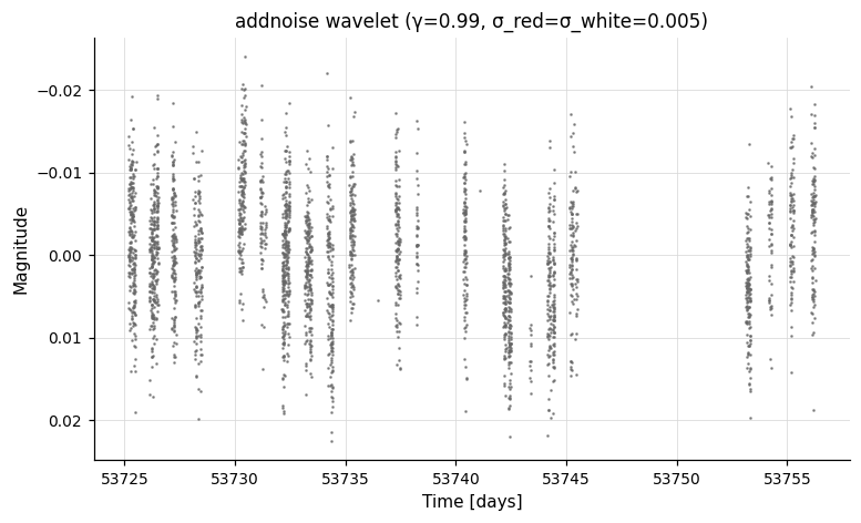
# Simulate wavelet (1/f-like) red noise + white noise
# (`gamma` sets the spectral-slope exponent; 2 ≈ 1/f^2 random walk)
result = lc_blank.addnoise(noise_type="wavelet", gamma=2.0,
                           sig_red=0.005, sig_white=0.005)
noisy_lc = result.lc

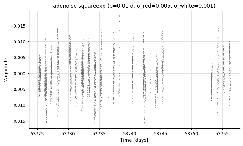
# Squared-exponential red noise with 0.01-day correlation timescale
result2 = lc_blank.addnoise(noise_type="squareexp", rho=0.01,
                            sig_red=0.005, sig_white=0.001)

---

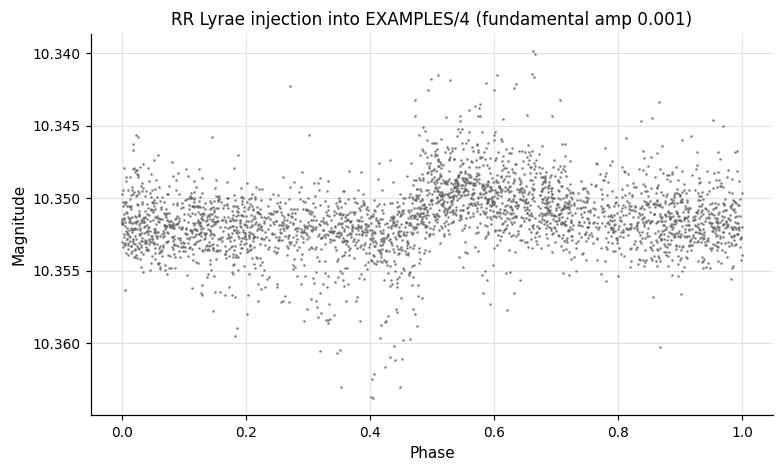
Injectharm — Inject a harmonic signal

Syntax

cmd.Injectharm(period, amplitude, nharm=1, phase=0.0,
               nsubharm=0, save_model=False)

Description

Inject a Fourier-series signal (sinusoid plus optional harmonics and sub-harmonics) into the light curve, primarily for injection-recovery tests. The injected model is

A_1·cos(2π·(t/P + φ_1))
  + Σ_{k=2..nharm} A_k·cos(2π·(t·k/P + φ_k))
  + Σ_{k=2..nsubharm+1} A_k·cos(2π·(t/(k·P) + φ_k))

period accepts a float (emits fix) or a string passed through verbatim — for example "logrand 1.0 5.0" for a log-uniform random period or "rand 0.5 5.0" for uniform random. amplitude accepts a float (ampfix), a bare-identifier string (ampvar), or an expression string (ampexpr). The wrapper exposes only the most common modes: for amprand, amplist, period-list, or period-rand modes, use cmd.Raw().

CLI equivalent: -Injectharm.

Parameters

Parameter	Type	Description
period	float or str	Period of the injected signal. Float → "fix val". String passes through (e.g. "rand 1.0 5.0", "logrand 0.5 5.0", "randfreq …", "lograndfreq …", "list").
amplitude	float or str	Per-harmonic amplitude. Float → "ampfix val". Bare-identifier string → "ampvar name"; other strings → "ampexpr expr" (e.g. "amplogrand 0.01 0.1").
nharm	int	Number of harmonics including the fundamental (≥ 1). The CLI receives Nharm = nharm − 1.
phase	float or str	Initial phase of each harmonic (0–1). Same float / var / expr forms as amplitude (uses phasefix / phasevar / phaseexpr); "phaserand" is accepted as a string for a uniform random draw.
nsubharm	int	Number of sub-harmonics. Each sub-harmonic uses the same amplitude / phase spec as the fundamental. Pass cmd.Raw() if you need per-sub-harmonic amplitudes or phases.
save_model	bool, str, or Output	Write the injected model as a .injectharm.model file. True captures as result.files["Injectharm_model_N"]. See Auxiliary output files.

Output

Suffix N is the 0-indexed pipeline command position:

Column	Description
Injectharm_Period_N	Injected period (days).
Injectharm_Fundamental_Amp_N	Amplitude of the fundamental.
Injectharm_Fundamental_Phase_N	Phase of the fundamental.
Injectharm_Harm_k_Amp_N, Injectharm_Harm_k_Phase_N	Amplitude and phase of harmonic k (for k = 2 … nharm).
Injectharm_Subharm_k_Amp_N, Injectharm_Subharm_k_Phase_N	Amplitude and phase of sub-harmonic k (for k = 2 … nsubharm + 1).

When save_model is set:

File key	Description
result.files["Injectharm_model_N"]	DataFrame of the injected model light curve (suffix .injectharm.model).

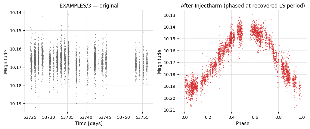
Examples

lc = vt.LightCurve.from_file("EXAMPLES/3")

# Inject a sine wave at a random log-uniform period, then try to recover it.
# `logrand`, `amplogrand`, and `phaserand` are vartools-side random draws that
# create scalar variables on the LC — we use a single Pipeline so those
# variables stay in the same invocation as the recovery step.
result = (vt.Pipeline()
        .Injectharm(period="logrand 1.0 5.0",
                   amplitude="amplogrand 0.001 0.1",
                   nharm=1, phase="phaserand",
                   save_model=True)
        .LS(0.5, 10.0, 0.1, npeaks=1)).run(lc)
print(result.vars["Injectharm_Period_0"])   # injected period
print(result.vars["LS_Period_1_1"])         # recovered period

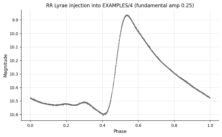
The same script with the canonical RR-Lyrae harmonic coefficients (and the fundamental amplitude reduced) shows the multi-harmonic shape directly:

---

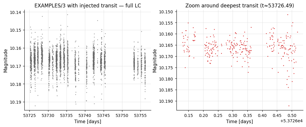
Injecttransit — Inject a transit signal

Syntax

cmd.Injecttransit(period, Rp, Mp, phase, sini, Mstar, Rstar,
                  e=0.0, omega=0.0,
                  hk=False, h=0.0, k=0.0,
                  dilute=None,
                  ld_type="quad", ld_coeffs=None, save_model=False)

Description

Inject a Mandel-Agol limb-darkened transit signal into the light curve. Each physical parameter accepts a float (the wrapper emits <prefix>fix val) or a string passed through verbatim — strings can use any of the CLI source keywords (Plogrand, Plist, Pexpr, phaserand, sinirand, …). Eccentricity is supplied either as (e, omega) (default) or as (h, k) when hk=True. Limb darkening is either quadratic (ld_type="quad", two coefficients) or non-linear (ld_type="nonlin", four coefficients).

CLI equivalent: -Injecttransit.

Parameters

Parameter	Type	Description
period	float or str	Orbital period (days). Float → "Pfix val". String passthrough (e.g. "Plogrand 0.2 2.0", "Plist").
Rp	float or str	Planet radius (Jupiter radii). Float → "Rpfix val" (e.g. "Rplogrand 0.05 0.15").
Mp	float or str	Planet mass (Jupiter masses).
phase	float or str	Phase of transit centre (0–1). Common string form: "phaserand".
sini	float or str	Sine of orbital inclination. Common string form: "sinirand" (uniform-orientation draw constrained to produce a transit).
Mstar	float or str	Stellar mass (M☉).
Rstar	float or str	Stellar radius (R☉).
e	float or str	Eccentricity (used with the default eomega mode).
omega	float or str	Argument of periastron in degrees (default mode).
hk	bool	When True, switch to (h, k) parameterisation: h = e·sin(ω), k = e·cos(ω).
h, k	float or str	Used when hk=True.
dilute	float, str, or None	Optional dilution factor (flux fraction from the target). Float → ["dilute", "fix", val]; string passthrough (e.g. "list").
ld_type	str	"quad" (2 coefficients) or "nonlin" (4 coefficients).
ld_coeffs	list of float	Limb-darkening coefficients. Default [0.3, 0.3].
save_model	bool, str, or Output	Write the injected model. True captures as result.files["Injecttransit_model_N"].

Output

Suffix N is the 0-indexed pipeline command position:

Column	Description
Injecttransit_Period_N	Injected period (days).
Injecttransit_Rp_N	Planet radius (Jupiter radii).
Injecttransit_Mp_N	Planet mass (Jupiter masses).
Injecttransit_phase_N	Injected phase.
Injecttransit_sin_i_N	Injected sin i.
Injecttransit_h_N, Injecttransit_k_N	Eccentricity components (only when hk=False; values are the supplied e, omega).
Injecttransit_e_N, Injecttransit_omega_N	Eccentricity components (only when hk=True; values are the supplied h, k).
Injecttransit_Mstar_N	Stellar mass (M☉).
Injecttransit_Rstar_N	Stellar radius (R☉).
Injecttransit_ld_k_N	Limb-darkening coefficient k (1 to Nld).

When save_model is set:

File key	Description
result.files["Injecttransit_model_N"]	DataFrame of the injected model light curve (suffix .injecttransit.model).

Examples

lc = vt.LightCurve.from_file("EXAMPLES/4")

# Inject a Jupiter-sized transit at a random period, then search with BLS.
# As with Injectharm, the per-LC random draws (`Plogrand`, `phaserand`, …) are
# scalar-variables produced inside vartools, so we run inject + recover in a
# single Pipeline invocation.
result = (vt.Pipeline()
        .Injecttransit(
            period="Plogrand 0.2 2.0",
            Rp="Rpfix 0.1",     # Rp/R*
            Mp="Mpfix 0.001",   # M_sun
            phase="phaserand",
            sini="sinirand",
            Mstar="Mstarfix 1.0",
            Rstar="Rstarfix 1.0",
            ld_type="quad",
            ld_coeffs=[0.3471, 0.3180],
            save_model=True,
        )
        .BLS(0.1, 5.0, rmin=0.01, rmax=0.1, nbins=200, nfreq=20000, npeaks=1)).run(lc)
print(result.vars["Injecttransit_Period_0"])   # injected period
print(result.vars["BLS_Period_1_1"])           # recovered period

---

copylc — Duplicate the light curve in-memory

Syntax

cmd.copylc(ncopies)

Description

Replicate the current light curve ncopies times in memory. Each copy is processed independently by all subsequent pipeline commands; the per-LC output table is replicated for every copy. Each copy's name has the suffix _copy$copycommandnum.$copynum appended, where $copycommandnum is the index of the copylc command and $copynum runs from 0 to ncopies − 1.

A common use is bootstrap / noise-replica Monte Carlo, where the same input is shifted into many parallel replicas that can be analysed by the downstream pipeline.

copylc cannot be used together with the -readall global option.

CLI equivalent: -copylc.

Parameters

Parameter	Type	Description
ncopies	int	Number of copies to create.

Output

copylc does not emit per-LC output columns of its own; instead it expands the output table by a factor of ncopies + 1. Downstream commands' columns are reported once per copy.

Example

lc = vt.LightCurve.from_file("EXAMPLES/2")
pipe_bs = (vt.Pipeline()
        .LS(0.1, 10.0, 0.1, npeaks=1)
        .copylc(100)
        .expr("mag=err*gauss()")
        .LS(0.1, 10.0, 0.1, npeaks=1))
batch_bs = pipe_bs.run_batch([lc])

---