Period finding
Run a Lomb-Scargle search on a light curve, then fit a single sinusoid at the
recovered period. EXAMPLES/2 has a 1.2354-day, 0.05 mag sine injected into
it; the LS+harmonic fit should recover a peak-to-peak amplitude of ~0.1 mag.
Command line
./vartools -i EXAMPLES/2 \
    -LS 1.0 2.0 0.01 1 0 \
    -harmonicfilter ls 0 0 1 EXAMPLES/OUTDIR1 \
    -oneline
Name                                       = EXAMPLES/2
LS_Period_1_0                              =     1.23538924
Log10_LS_Prob_1_0                          = -4199.53506
LS_Periodogram_Value_1_0                   =    0.99711
LS_SNR_1_0                                 =   20.55841
HarmonicFilter_Mean_Mag_1                  =  10.12192
HarmonicFilter_Period_1_1                  =     1.23538924
HarmonicFilter_Per1_Fundamental_Sincoeff_1 =  -0.04836
HarmonicFilter_Per1_Fundamental_Coscoeff_1 =  -0.01286
HarmonicFilter_Per1_Amplitude_1            =   0.10009
Python
import pyvartools as vt
from pyvartools import commands as cmd

lc = vt.LightCurve.from_file("EXAMPLES/2")

result = (vt.Pipeline()
        .LS(1.0, 2.0, 0.01, npeaks=1, save_periodogram=False)
        .harmonicfilter(period="ls", nharm=0, nsubharm=0)).run(lc)

print(result.vars)
Name                                                   2
LS_Period_1_0                                   1.235389
Log10_LS_Prob_1_0                            -4199.53506
LS_Periodogram_Value_1_0                         0.99711
LS_SNR_1_0                                      20.55841
HarmonicFilter_Mean_Mag_1                       10.12192
HarmonicFilter_Period_1_1                       1.235389
HarmonicFilter_Per1_Fundamental_Sincoeff_1      -0.04836
HarmonicFilter_Per1_Fundamental_Coscoeff_1      -0.01286
HarmonicFilter_Per1_Amplitude_1                  0.10009
Capture and plot the LS periodogram
Capture the full LS frequency-power spectrum for EXAMPLES/2, read it into
Python as a DataFrame, and plot power vs. period.
Command line
The 1 EXAMPLES/OUTDIR1 at the end of the -LS args enables periodogram
output and writes it to EXAMPLES/OUTDIR1/2.ls:
# Column 1 = Frequency in cycles per input light curve time unit.
# Column 2 = Unnormalized P(omega) (equation 5 of Zechmeister &
#            K\"urster 2009, A&A, 496, 577).
# Column 3 = Logarithm of the false alarm probability.
0.10000931941552052 0.053061184352138094 -2148.7692206324959
0.10004060923970099 0.052928767751820608 -2147.0684086900499
0.10007189906388148 0.052797859472316708 -2145.3766960921931
...
Python
save_periodogram=True captures the spectrum as a pandas DataFrame in
result.files["LS_periodogram_0"] (three columns: frequency, power, log₁₀
FAP). The example plots power against period with the LS peak marked.
import matplotlib
matplotlib.use("Agg")           # headless backend; drop for interactive use
import matplotlib.pyplot as plt
import pyvartools as vt

lc = vt.LightCurve.from_file("EXAMPLES/2")
result = lc.LS(0.5, 10.0, 0.001, save_periodogram=True)

pgram = result.files["LS_periodogram_0"]
print(pgram.head())
print(f"shape: {pgram.shape}")

fig, ax = plt.subplots(figsize=(7, 3))
period = 1.0 / pgram[0]
ax.plot(period, pgram[1], lw=0.5)
ax.set_xscale("log")
ax.set_xlabel("Period (days)")
ax.set_ylabel("LS power")
ax.axvline(result.varobjs.LS.Period_1, color="C1", lw=1,
           label=f"peak P = {result.varobjs.LS.Period_1:.4f} d")
ax.legend()
fig.tight_layout()
fig.savefig("/tmp/ls_periodogram.png", dpi=100)
          0         1            2
0  0.100009  0.053061 -2148.769221
1  0.100041  0.052929 -2147.068409
2  0.100074  0.052798 -2145.376696
3  0.100106  0.052668 -2143.694210
4  0.100138  0.052539 -2142.021078
shape: (59104, 3)
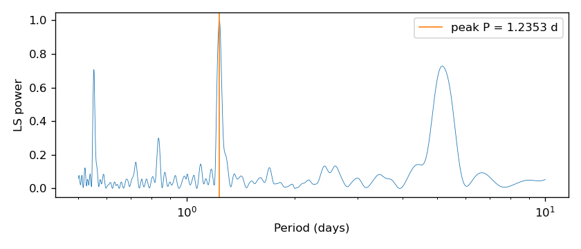
The DataFrame has 59 104 rows spanning 0.10–2.0 cycles/day. Column indices are integers because the vartools periodogram file has no header row — column 0 is frequency, column 1 is power, column 2 is log₁₀ false-alarm probability.
AoV on a light curve with an injected eclipsing-binary signal
Inject a realistic detached eclipsing-binary signal into EXAMPLES/4 using
the JKTEBOP model (shipped as a USERLIB extension), then run three
period-finders on the result to compare how each responds to a non-sinusoidal
signal with two dips per orbit.
The injection uses a 1.7345 d orbit, a/(R₁+R₂) = 8 (so sum of fractional
radii r₁+r₂ = 0.125), R₂/R₁ = 0.8, mass ratio 0.8, surface-brightness ratio
J₂/J₁ = 0.25, central eclipses (bimpact = 0), circular orbit, and
quadratic limb darkening with coefficients (0.6, 0.2) on both stars.
Command line
Shell variable T0 is the first observation in EXAMPLES/4 (53725.17392),
which we use as the reference epoch so the first primary eclipse lands at
the start of the light curve.
T0=53725.17392
./vartools \
    -L /home/jhartman/SVN/HATpipe/data/vartools/USERLIBS/jktebop.so \
    -i EXAMPLES/4 \
    -jktebop inject \
        Period fix 1.7345 T0 fix $T0 \
        r1+r2 fix 0.125 r2/r1 fix 0.8 M2/M1 fix 0.8 J2/J1 fix 0.25 \
        bimpact fix 0.0 esinomega fix 0.0 ecosomega fix 0.0 \
        LD1 quad fix 0.6 0.2 \
        LD2 quad fix 0.6 0.2 \
    -LS 0.5 10.0 0.0005 1 0 \
    -aov Nbin 100 0.5 10.0 0.1 0.001 1 0 \
    -aov_harm 50 0.5 10.0 0.1 0.001 1 0 \
    -oneline
-aov uses Nbin 100 instead of the default 8 — more phase bins mean the
two narrow eclipses fall inside their own bins, instead of being diluted
into the sinusoid-scale bin grid. -aov_harm uses Nharm = 50 — far more
harmonics than typical for a sinusoidal signal, but appropriate for the
sharp, narrow eclipse profile of an EB.
Name                       = EXAMPLES/4
Jktebop_PERIOD_0           = 1.73450
Jktebop_T0_0               = 53725.17392
Jktebop_R1+R2_0            = 0.125
Jktebop_R2/R1_0            = 0.8
Jktebop_M2/M1_0            = 0.8
Jktebop_J2/J1_0            = 0.25
Jktebop_BIMPACT_0          = 0
Jktebop_INCLINATION_0      = 90
LS_Period_1_1              =     0.86992186
Log10_LS_Prob_1_1          =  -55.14150
LS_SNR_1_1                 =    4.80510
Period_1_2                 =     1.73441598
AOV_1_2                    =  487.90254
AOV_SNR_1_2                =   67.78358
Period_1_3                 =     1.73451269
AOV_HARM_1_3               =  5317.63
AOV_HARM_SNR_1_3           =   415.72
Lomb-Scargle finds the half-period harmonic (0.870 d) at SNR 4.8 because a sinusoid at P/2 matches the symmetric primary-secondary structure about as well as one at P. Both AoV variants recover the true injected period (1.7345 d). The higher bin/harmonic counts are the key: a coarse model picks up the P/2 harmonic.
Python
The typed cmd.jktebop(...) wrapper is auto-loaded from the installed
userlibs directory, so no lib_path= argument is needed in this example.
import pyvartools as vt
from pyvartools import commands as cmd

lc = vt.LightCurve.from_file("EXAMPLES/4")
T0 = float(lc.t.min())

result = (vt.Pipeline()
        .jktebop(
            "inject",
            Period=1.7345, T0=T0,
            r1_r2=0.125, r2_r1=0.8, M2_M1=0.8, J2_J1=0.25,
            bimpact=0.0, esinomega=0.0, ecosomega=0.0,
            LD1_law="quad", LD1_coeffs=(0.6, 0.2),
            LD2_law="quad", LD2_coeffs=(0.6, 0.2),
        )
        .LS(0.5, 10.0, 0.0005, npeaks=1)
        .aov(0.5, 10.0, 0.1, finetune=0.001, nbin=100, npeaks=1)
        .aov_harm(nharm=50, minp=0.5, maxp=10.0, subsample=0.1,
                 finetune=0.001, npeaks=1)).run(lc)

print(f"injected : 1.73450 d (P/2 = 0.86725 d)")
print(f"LS       : P={result.vars['LS_Period_1_1']:.5f} d   "
      f"SNR={result.vars['LS_SNR_1_1']:.2f}")
print(f"AoV      : P={result.vars['Period_1_2']:.5f} d   "
      f"SNR={result.vars['AOV_SNR_1_2']:.2f}")
print(f"AoV_harm : P={result.vars['Period_1_3']:.5f} d   "
      f"SNR={result.vars['AOV_HARM_SNR_1_3']:.2f}")
injected : 1.73450 d (P/2 = 0.86725 d)
LS       : P=0.86992 d   SNR=4.80
AoV      : P=1.73442 d   SNR=67.78
AoV_harm : P=1.73451 d   SNR=415.72
The typed jktebop wrapper's attributes (r1_r2, r2_r1, M2_M1,
J2_J1) use underscores because + and / can't appear in Python
identifiers. The CLI-side r1+r2, r2/r1, etc. are emitted automatically.
"inject" mode is first-positional; the parameter defaults match the CLI's
fix keyword unless you pass vary_Period=True etc. to free them in a
fit (see the Model Fitting → jktebop command reference).
Phase-folded at the AoV-recovered period
Inject, find the period, and phase-fold the light curve in one pipeline
using -Phase. The fold is placed on the AoV-recovered period (1.73442 d)
with a quarter-period T0 offset so the primary eclipse sits at phase −0.25
and the secondary at +0.25, giving each dip its own breathing room in a
[−0.5, 0.5] x-axis.
-Phase stores the per-point phase in the LC vector variable ph via
phasevar; startphase -0.5 shifts the fold range from the default
[0, 1) to [−0.5, 0.5). The T0 expression references the AoV
command's native Period_1_1 output column. myT0 is set via -expr
listvar so it's available in the T0 expression. The variable ph
will be included in the captured output light curve, together with the
default variables t, mag, and err. Giving the key="folded"
option to cmd.o() allows access to the output light curve via
result.files["folded"].
import matplotlib
matplotlib.use("Agg")
import matplotlib.pyplot as plt
import pyvartools as vt
from pyvartools import commands as cmd

lc = vt.LightCurve.from_file("EXAMPLES/4")
T0 = float(lc.t.min())

result = (vt.Pipeline()
        .jktebop(
            "inject",
            Period=1.7345, T0=T0,
            r1_r2=0.125, r2_r1=0.8, M2_M1=0.8, J2_J1=0.25,
            bimpact=0.0, esinomega=0.0, ecosomega=0.0,
            LD1_law="quad", LD1_coeffs=(0.6, 0.2),
            LD2_law="quad", LD2_coeffs=(0.6, 0.2),
        )
        .aov(0.5, 10.0, 0.1, finetune=0.001, nbin=100, npeaks=1)
        .expr(f"myT0={T0}", vartype="listvar")
        .Phase(period="aov",
              T0="expr myT0+0.25*Period_1_1",
              phasevar="ph",
              startphase=-0.5)
        .o(capture=True, key="folded")).run(lc)

P_aov = float(result.varobjs.aov.Period_1)
df = result.files["folded"].to_dataframe()

fig, ax = plt.subplots(figsize=(7, 3.2))
ax.plot(df["ph"], df["mag"], ".", ms=1.2, color="C0")
ax.invert_yaxis()          # magnitude convention: brighter = lower y
ax.set_xlim(-0.5, 0.5)
ax.set_xlabel(f"Phase  (P = {P_aov:.5f} d, eclipses at ±0.25)")
ax.set_ylabel("mag")
fig.tight_layout()
fig.savefig("/tmp/eb_phased.png", dpi=120)
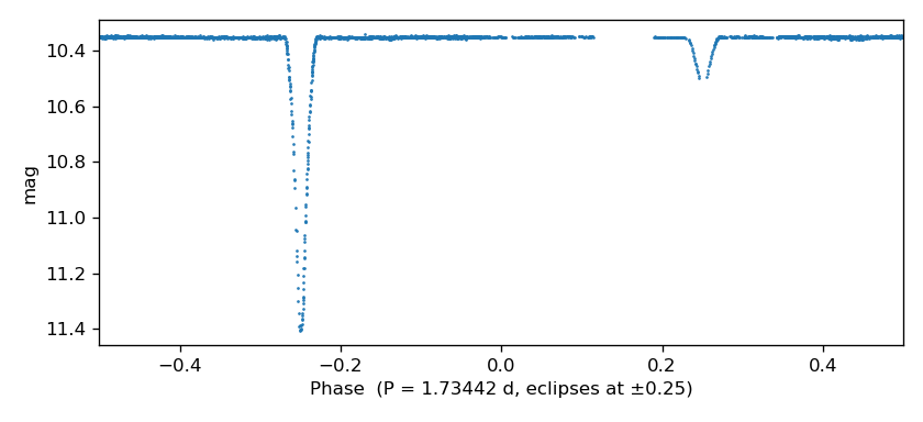
The above script produces this plot.
Notes
The 0 at the end of the -LS argument list disables periodogram output;
pass a directory path (or set save_periodogram=True in Python) to write the
frequency-power spectrum for plotting.
-harmonicfilter with ls picks up the top LS period from the prior command.
The three zeros after ls request fundamental-only (no harmonics, no
sub-harmonics, output the model LC with the best-fit sine in the third
column). The EXAMPLES/OUTDIR1 argument is the directory where the model LC
is written as EXAMPLES/OUTDIR1/2.harmonicfilter.model.
-oneline reformats the one-row-per-LC default into one-statistic-per-line
— handy for single-LC runs.
Useful variants:
- Save a periodogram for plotting: replace the
0after the peak count withoperiodogram EXAMPLES/OUTDIR1in the CLI, or setsave_periodogram=Trueincmd.LS(...). Withsave_periodogram=Truethe periodogram is available as a DataFrame viaresult.files["LS_periodogram_0"]. - Report more peaks: change the
1after the frequency step (andnpeaks=1) to a larger number; the output columns becomeLS_Period_1_0throughLS_Period_N_0. - AoV / multi-harmonic AoV: swap
-LSfor-aovor-aov_harm NHARM; the rest of the pipeline is identical. - For some non-sinusoidal signals,
-aov_harmcan recover periods more reliably than Lomb-Scargle. - Sigma-clip first to stop outliers from dominating the periodogram:
prepend
-clip 5.0 1(CLI) orcmd.clip(5.0, iterative=True)(Python).