Light Curve Manipulation¶

Commands that transform, resample, or reinterpret the light curve in-memory — column arithmetic, time manipulation, unit conversions, and Fourier transforms of evenly-sampled data.

`sortlc` — Sort observations¶

Syntax

cmd.sortlc(var=None, reverse=False)

Description

Sort the light curve observations. By default, observations are sorted by time (ascending). Use var to sort by another named variable (e.g. "mag") and reverse=True to sort in descending order. If a subsequent command requires time-sorted data, vartools automatically restores time order at the start of that command.

CLI equivalent: -sortlc.

Parameters

Parameter	Type	Description
`var`	`str` or `None`	Name of the variable to sort by. `None` (default) sorts by time.
`reverse`	`bool`	Sort in descending order instead of ascending.

Output

Modifies the LC in-place: reorders all per-observation vectors by the chosen sort key; no output statistics.

Examples

lc = vt.LightCurve.from_file("EXAMPLES/2")

# Reverse-time sort
(vt.Pipeline().sortlc(reverse=True)
              .o("EXAMPLES/OUTDIR1/2.rev.txt")).run(lc)

# Sort by magnitude (brightest first)
(vt.Pipeline().sortlc(var="mag")
              .o("EXAMPLES/OUTDIR1/2.magsorted.txt")).run(lc)

`binlc` — Bin in time¶

Syntax

cmd.binlc(method="average", binsize=None, nbins=None,
          time_output="tcenter", bincolumns=None,
          bincolumnsonly=False, T0=None, firstbinshift=None,
          maskpoints=None)

Description

Bin the light curve in time (or in phase, when applied after a Phase command). All light-curve vectors are binned together using the chosen statistic. Specify the bin width via binsize or the total number of equal-width bins via nbins (one of the two is required).

CLI equivalent: -binlc.

Parameters

Parameter	Type	Description
`method`	`str`	Combination statistic: `"average"`, `"median"`, or `"weightedaverage"`.
`binsize`	`float` or `str`	Bin width in time (or phase) units. Either `binsize` or `nbins` must be provided. Accepts variable names and expressions.
`nbins`	`int` or `str`	Number of equal-width bins to divide the time span into (alternative to `binsize`).
`time_output`	`str`	Output time for each bin: `"tcenter"`, `"taverage"`, `"tmedian"`, or `"tnoshrink"` (replace each point with its binned value without shrinking the LC).
`bincolumns`	`str` or `None`	Override the binning statistic for specific named columns, e.g. `"col1,col2:median"`.
`bincolumnsonly`	`bool`	With `time_output="tnoshrink"`, restrict replacement to columns listed in `bincolumns`.
`T0`	`float`, `str`, or `None`	Reference time for bin-edge alignment. A float emits `"fix T0"`; a string is split and forwarded verbatim (e.g. `"list"` or `"fixcolumn colname"`).
`firstbinshift`	`float`, `str`, or `None`	Shift the first bin edge by this amount. Accepts variable/expression forms.
`maskpoints`	`str` or `None`	Mask variable; only points with `maskvar > 0` contribute. Masked-out points still receive the binned value when `tnoshrink` is active.

Output

Modifies the LC in-place: replaces all per-observation vectors with their binned values (the LC length is reduced unless time_output="tnoshrink"); no output statistics.

Examples

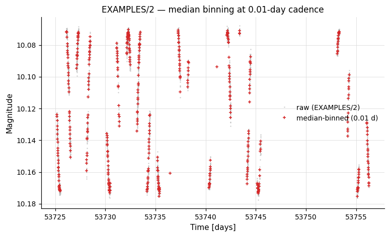
lc = vt.LightCurve.from_file("EXAMPLES/2")

# Bin in time with 0.01-day bins (median combination)
result = lc.binlc(method="median", binsize=0.01)
binned_lc = result.lc

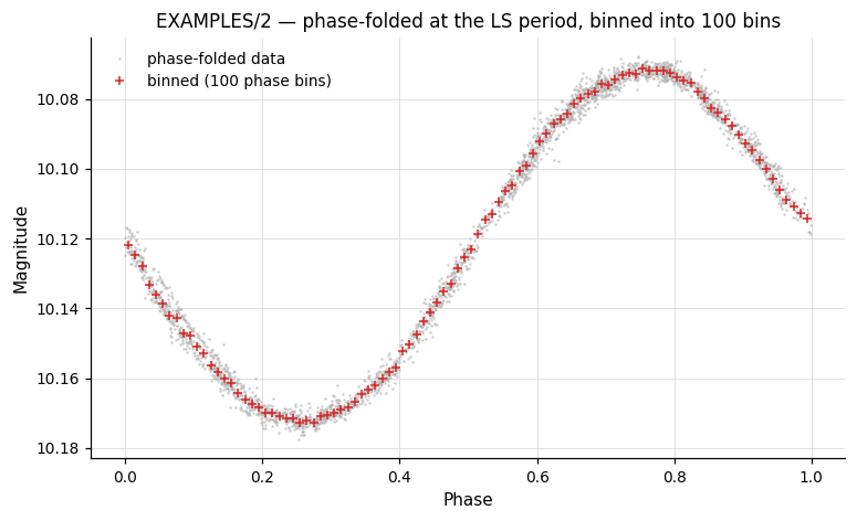
# Phase-fold then bin into 100 phase bins.  `cmd.Phase(period="ls")`
# back-references the prior LS and works both in a single Pipeline and
# across chain steps.
pipe = (vt.Pipeline()
        .LS(0.1, 10.0, 0.1, npeaks=1)
        .Phase(period="ls")
        .binlc(method="median", nbins=100))
result = pipe.run(lc, capture_lc=True)
phase_binned_lc = result.lc

Median-binned EXAMPLES/2 EXAMPLES/2 phase-folded + binned at the LS period

`Phase` — Phase-fold the light curve¶

Syntax

cmd.Phase(period="ls", T0=None, phasevar=None, startphase=None)

Description

Replace the time axis of the light curve with its phase, computed as ((t − T0) mod P) / P, and sort by phase. Phases run from 0 to 1 by default (or from startphase to startphase + 1). After Phase, time-based binning commands like binlc operate in phase space.

CLI equivalent: -Phase.

Parameters

Parameter	Type	Description
`period`	`float` or `str`	Period to fold on. Accepts a number, or a back-reference keyword: `"ls"`, `"aov"`, `"bls"`, `"fixcolumn NAME"`, `"list"`.
`T0`	`float`, `str`, or `None`	Reference epoch. Accepts a number, or `"bls <phase_offset>"` to derive `T0 = Tc − phase_offset · Period` from the prior BLS result (e.g. `T0="bls 0.5"` puts mid-transit at phase 0.5). Default: the earliest time in the LC.
`phasevar`	`str` or `None`	Name of the output phase variable. Default: overwrites `t`.
`startphase`	`float` or `None`	Starting phase (default 0). Phase range becomes `[startphase, startphase + 1)`.

Back-references work across chain steps

period accepts "ls", "aov", "bls", and "fixcolumn NAME"; T0 accepts the "bls <phase_offset>" form. All of these resolve correctly inside a single Pipeline and across chain boundaries (e.g. lc.LS(...).Phase(period="ls") or lc.BLS(...).Phase(period="bls", T0="bls 0.5")). In batch-chain mode the resolved values become per-LC, so each light curve is folded on its own period / Tc. Missing prior command → LookupError.

Output

Modifies the LC in-place: replaces t (or writes to phasevar) with phase values and re-sorts the LC; no output statistics.

Examples

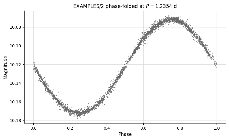
lc = vt.LightCurve.from_file("EXAMPLES/2")

# Phase-fold at a known period
result = lc.Phase(period=1.2354)
phased_lc = result.lc   # time column replaced by orbital phase

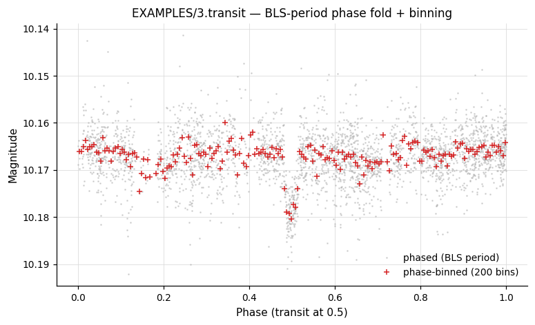
# Use period found by BLS, set mid-transit at phase 0.5.
# `period="bls"` and `T0="bls 0.5"` work across the chain boundary —
# pyvartools reads BLS_Period_1 / BLS_Tc_1 from the prior result.
lc_transit = vt.LightCurve.from_file("EXAMPLES/3.transit")
result = (
    lc_transit
        .BLS(0.5, 5.0, rmin=0.01, rmax=0.1, nbins=200, nfreq=20000, npeaks=1)
        .Phase(period="bls", T0="bls 0.5")
        .binlc(method="median", nbins=200)
)
phase_binned_lc = result.lc

Phase-folded EXAMPLES/2 at P=1.2354 d EXAMPLES/3.transit phased + binned at the BLS period

`resample` — Resample onto a new time grid¶

Syntax

cmd.resample(method="linear",
             left=None, right=None,
             nbreaks=None, order=None,
             file_times=None, file_column=None,
             list_column=None, t_column=None,
             gaps=None,
             tstart=None, tstop=None, delt=None, Npoints=None)

Description

Resample the light curve onto a new time base by interpolating all light-curve vectors. The default output grid runs from the first to the last observed time with a step equal to the minimum observed time separation. Specify the new grid with delt (step size), Npoints (number of points), or file_times (times read from a file). String-type columns (e.g. image IDs) are always resampled with the "nearest" method.

CLI equivalent: -resample.

Parameters

Parameter	Type	Description
`method`	`str`	Interpolation method: `"nearest"`, `"linear"`, `"spline"`, `"splinemonotonic"`, or `"bspline"`.
`left`	`float` or `None`	First-derivative boundary condition at the left edge of the spline. Only for `method="spline"` (or `"splinemonotonic"`).
`right`	`float` or `None`	First-derivative boundary condition at the right edge of the spline.
`nbreaks`	`int` or `None`	Number of interior break points for B-spline fitting. Only for `method="bspline"`. If `< 2`, breaks are increased until χ²/dof ≤ 1 (can be slow).
`order`	`int` or `None`	Polynomial order of the B-spline (only for `method="bspline"`).
`file_times`	`str` or `None`	Source for the new time grid. Either: (a) a path string → resample to the times in that file (the same grid is used for every LC), or (b) the literal `"list"` → resample, per LC, to the times in a file whose path is read from a column of the input list file (list-mode runs only).
`file_column`	`int` or `None`	Legacy alias for `t_column` in path mode. Prefer `t_column`.
`list_column`	`int` or `None`	Only with `file_times="list"`. 1-based column number in the input list file that holds the per-LC time-grid filename. When omitted, the next unused list-file column is consumed.
`t_column`	`int` or `None`	1-based column number in the time-grid file that holds the time values. Defaults to `1`.
`gaps`	`str` or `None`	Gap-handling spec, e.g. `"percentile_sep 80 bspline"` — switches interpolation method beyond a separation threshold.
`tstart`, `tstop`	`float`, `str`, or `None`	Start and stop of the new time grid. Accepts variable/expression/per-LC forms.
`delt`	`float`, `str`, or `None`	Time step of the new grid.
`Npoints`	`int`, `str`, or `None`	Number of points in the new grid (alternative to `delt`).

Output

Modifies the LC in-place: replaces every per-observation vector by interpolating onto the new time grid; no output statistics.

Examples

lc = vt.LightCurve.from_file("EXAMPLES/2")

# Linear interpolation with default time grid
result = lc.resample(method="linear")

# Monotonic spline onto a fixed time grid with 1000 points
result2 = lc.resample(method="splinemonotonic",
                      tstart=53726, tstop=53756, Npoints=1000)

# B-spline with 20 break points, order 3
result3 = lc.resample(method="bspline", nbreaks=20, order=3, Npoints=500)

# List-form back-resampling: bin to a coarse grid, then resample back
# onto each LC's *original* time grid.  list_column=1 says read the
# time-grid filename from column 1 of the list file (the LC path
# itself); t_column=1 says read times from column 1 of that file.
import os, tempfile
list_path = os.path.join(tempfile.mkdtemp(), "lclist.txt")
with open(list_path, "w") as f:
    f.write("EXAMPLES/2\n")
batch = (vt.Pipeline()
         .binlc(method="average", binsize=0.05)
         .resample(method="linear",
                   file_times="list", list_column=1, t_column=1)
         .rms()
         ).run_filelist(list_path, capture_lc=True)
print(batch.vars[["Name", "RMS_2"]])

`expr` — Analytic expression¶

Syntax

cmd.expr(expression, vartype=None, outputcolumn=False)

Description

Evaluate an analytic expression and assign the result to a named variable. The expression has the form varname=formula, e.g. "residual=mag-model". If the variable does not yet exist it is created as a per-observation light-curve vector by default; the optional vartype keyword selects another lifetime — see the vartype aggregation note below.

The expression engine supports aggregate functions like mean(mag), stddev(mag), pct(mag, 95.0), and filtering like mean(mag, t>53730). See the Analytic Expressions reference for the complete list of operators, functions, and constants.

Operator names

The expression grammar follows C, not NumPy: modulo is t%P (not mod(t, P)), power is mag^2 (not mag**2), and there is no np. prefix on functions (sqrt, log, sin, etc. are bare names).

CLI equivalent: -expr.

Parameters

Parameter	Type	Description
`expression`	`str`	Expression of the form `varname=formula`. The LHS may reference any existing light-curve vector, scalar from prior commands, or output-column header name.
`vartype`	`str` or `None`	Type of the LHS variable: `None` (per-observation, default), `"listvar"` (per-star), `"scalar"` (per-thread), or `"const"` (global constant). See `vartype` and aggregate functions. If the variable already exists, its type is preserved regardless of this setting.
`outputcolumn`	`bool`	If `True`, expose the LHS variable's value as a column in the result table (named `Expr_<varname>_<command-index>`). Only valid when `vartype` is `"listvar"`, `"scalar"`, or `"const"`; passing `outputcolumn=True` with `vartype=None` raises `ValueError` at construction (the value would otherwise be per-observation, not a single column). Default `False`.

Output

Modifies the LC in-place: creates or updates the named variable. Emits no statistics columns by default. When outputcolumn=True, an Expr_<varname>_<command-index> column is added to the result table.

Examples

lc = vt.LightCurve.from_file("EXAMPLES/1")

# Apply a mathematical transform in-place
result = lc.expr("mag=sqrt(mag+5)")

# Compute per-star mean magnitude using an aggregate function.
# `avg` is a `listvar` variable created inside vartools — it must be visible
# to the next `-expr` step, so these three commands share one Pipeline.
pipe = (vt.Pipeline()
        .expr("avg=mean(mag)", vartype="listvar")
        .expr("dmag=mag-avg")
        .rms())
result = pipe.run(lc)

# Same as above but expose the per-star mean in the result table.
# `outputcolumn=True` adds a column named `Expr_avg_<command-index>`.
pipe = (vt.Pipeline()
        .expr("avg=mean(mag)", vartype="listvar", outputcolumn=True)
        .expr("dmag=mag-avg")
        .stats("dmag", "median,stddev"))
result = pipe.run(lc)
print(result.vars["Expr_avg_0"])         # the per-star mean magnitude

# Define a global constant and use it
pipe = (vt.Pipeline()
        .expr("zp=25.0", vartype="const")
        .expr("flux=10^(-0.4*(mag-zp))"))

# Convert to flux, normalise by median, then compute statistics
pipe = (vt.Pipeline()
        .expr("flux=10^(-0.4*(mag-25.0))")
        .stats("flux", ["median"])
        .expr("flux=flux/STATS_flux_MEDIAN_1")
        .stats(["flux", "mag"], ["median", "stddev"]))
result = pipe.run(lc)
print(result.vars["STATS_flux_MEDIAN_1"])   # original median flux
print(result.vars["STATS_flux_MEDIAN_3"])   # ≈ 1.0 after normalisation

`FFT` / `IFFT` — Fast Fourier Transform¶

Syntax

cmd.FFT(input_real, input_imag, output_real, output_imag)
cmd.IFFT(input_real, input_imag, output_real, output_imag)

Description

Compute the Fast Fourier Transform (FFT) or inverse Fast Fourier Transform (IFFT) of two named light-curve variables (real and imaginary parts), using GSL's gsl_fft_complex_forward() / ..._backward(). Element k of the transform corresponds to frequency k / (N · Δ) for k < N/2 (negative frequencies for k > N/2), where Δ is the assumed uniform time step and N is the number of points.

Use "NULL" for either input component to substitute a zero vector; use "NULL" for either output component to discard that component.

CLI equivalent: -FFT / -IFFT.

Parameters

Parameter	Type	Description
`input_real`	`str`	Name of the LC vector holding the real part of the input signal, or `"NULL"`.
`input_imag`	`str`	Name of the LC vector holding the imaginary part, or `"NULL"`.
`output_real`	`str`	Variable name to store the real part of the transform, or `"NULL"`.
`output_imag`	`str`	Variable name to store the imaginary part of the transform, or `"NULL"`.

Output

Modifies the LC in-place: writes the transform into the named output variables; no output statistics.

Examples

lc = vt.LightCurve.from_file("EXAMPLES/11")

# High-pass Fourier filter on a uniformly sampled light curve
pipe = (vt.Pipeline()
        .FFT("mag", "NULL", "fftreal", "fftimag")
        .rms()
        .expr("fftreal=(NR>(Npoints_1/500.0))*(NR<(Npoints_1*499.0/500.0))*fftreal")
        .expr("fftimag=(NR>(Npoints_1/500.0))*(NR<(Npoints_1*499.0/500.0))*fftimag")
        .IFFT("fftreal", "fftimag", "mag_filter", "NULL"))
result = pipe.run(lc, capture_lc=True)

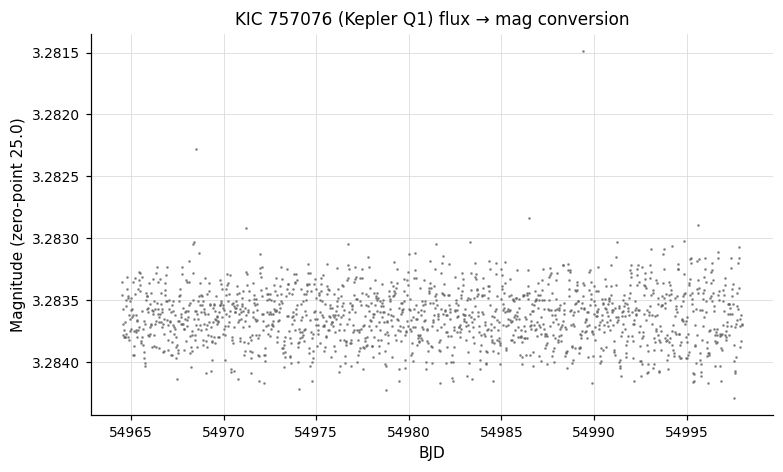
`difffluxtomag` / `fluxtomag` — Flux conversions¶

Syntax

cmd.difffluxtomag(mag_constant, offset=0.0, magcolumn=None)
cmd.fluxtomag(mag_constant, offset=0.0)

Description

Convert flux values to magnitudes:

fluxtomag — Convert absolute flux to magnitude using mag = mag_constant − 2.5·log10(flux) + offset.
difffluxtomag — Convert ISIS image-subtraction differential flux to magnitude using mag = mag_constant − 2.5·log10(ref_flux + diff_flux) + offset. Requires a list input where the reference magnitude of each star (after aperture correction) is supplied as an additional column.

mag_constant and offset accept numbers, variable names, or expression strings.

CLI equivalent: -fluxtomag / -difffluxtomag.

Parameters

Parameter	Type	Description
`mag_constant`	`float` or `str`	Magnitude corresponding to a flux of 1 ADU (zero-point).
`offset`	`float` or `str`	Additive constant applied to the output magnitudes.
`magcolumn`	`int` or `None`	(`difffluxtomag` only) Column in the input list containing the reference magnitude. Default: next available column.

Output

Modifies the LC in-place: replaces mag with the converted magnitude values; no output statistics.

Examples

# Synthesize a flux-unit light curve from an existing magnitude LC,
# then convert it back to magnitudes using `fluxtomag`.
import numpy as np

lc_mag = vt.LightCurve.from_file("EXAMPLES/2")
t, mag, err = lc_mag.t, lc_mag.mag, lc_mag.err
flux = 10.0 ** (-0.4 * (mag - 25.0))
lc_flux = vt.LightCurve.from_arrays(t, flux, err * flux * np.log(10) / 2.5)

# `mag_constant` is the zero-point magnitude (here 25.0, matching the
# synthesis above).
result = lc_flux.fluxtomag(25.0, offset=0.0)
print(result.lc.mag[:3])   # back to approximately the original values

KIC 757076 Q1 LC converted to magnitudes

`changeerror` — Rescale measurement uncertainties¶

Syntax

cmd.changeerror(maskpoints=None)

Description

Replace the formal per-point measurement uncertainties with the RMS of the light curve. Useful before χ² or MCMC fitting when the quoted uncertainties are known to be mis-calibrated, or when no formal errors are available.

CLI equivalent: -changeerror.

Parameters

Parameter	Type	Description
`maskpoints`	`str` or `None`	Mask variable; only points with `maskvar > 0` contribute to the RMS.

Output

Suffix N is the pipeline command index.

Column	Description
`Mean_Mag_N`	Mean magnitude of the light curve.
`RMS_N`	RMS of the light curve (the value the `err` column is replaced with).
`Npoints_N`	Number of points used.

The LC's err column is also modified in-place: every entry becomes the value reported as RMS_N.

Examples

lc = vt.LightCurve.from_file("EXAMPLES/4")
result = (
    lc.chi2()
      .changeerror()
      .chi2()
)
print(result.vars["Chi2_0"])   # 5.19874 (original)
print(result.vars["Chi2_2"])   # ≈ 1.0 (after rescaling errors to RMS)

`converttime` — Time system conversion¶

Syntax

cmd.converttime(input_format, output_format, ra=None, dec=None,
                input_subtract=None, output_subtract=None,
                input_sys=None, output_sys=None, ephemfile=None,
                leapsecfile=None)

Description

Convert the light curve's time column between Modified Julian Date (MJD), Julian Date (JD), Heliocentric Julian Date (HJD), and Barycentric Julian Date (BJD) systems. BJD conversion requires VARTOOLS to be linked to the JPL NAIF cspice library. The internal precision near J2000.0 is approximately 0.1 milliseconds. For HJD/BJD conversions, provide ra and dec in degrees.

CLI equivalent: -converttime.

Parameters

Parameter	Type	Description
`input_format`	`str`	Input time system: `"mjd"`, `"jd"`, `"hjd"`, or `"bjd"`.
`output_format`	`str`	Output time system.
`ra`	`float`, `str`, or `None`	Right ascension (deg) for HJD/BJD. A float emits `"radec fix ra dec"` (requires `dec`); a string is split and forwarded verbatim (e.g. `"list"`).
`dec`	`float` or `None`	Declination (deg), used together with a numeric `ra`.
`input_subtract`	`float` or `None`	Constant subtracted from the stored input times (e.g. `2400000` if input is `HJD-2400000`).
`output_subtract`	`float` or `None`	Constant subtracted from the output times.
`input_sys`	`str` or `None`	Input time system: `"tdb"` or `"utc"`. Default: UTC.
`output_sys`	`str` or `None`	Output time system: `"tdb"` or `"utc"`.
`ephemfile`	`str` or `None`	Path to a JPL ephemeris kernel (BJD/TDB conversions).
`leapsecfile`	`str` or `None`	Path to a leap-second kernel file.

Output

Modifies the LC in-place: replaces t with times in the requested system; no output statistics.

Examples

lc = vt.LightCurve.from_file("EXAMPLES/1")

# Convert JD (minus 2400000) to HJD for a known sky position
result = lc.converttime(
    input_format="jd",
    output_format="hjd",
    ra=88.079166,
    dec=32.5533,
    input_subtract=2400000.0,
)
hjd_lc = result.lc

`match` — Match against a catalog¶

Syntax

cmd.match(catalog, matchcolumn, addcolumns, missing="nanmissing",
          source="file", inlist_column=None, skipnum=None,
          skipchar=None, delimiter=None, opencommand=None)

Description

Perform a row-by-row match of an external data file to the light curve, merging columns from the catalog into the LC. The match is performed on a specified variable (by default the time t). Float/double columns are matched within the tolerance set by the global -jdtol; all other types are matched exactly. New variables are created from the catalog; existing variables are overwritten.

CLI equivalent: -match.

Parameters

Parameter	Type	Description
`catalog`	`str`	Path to the catalog file (FITS table for `.fits` extensions). Ignored when `source="inlist"`.
`source`	`str`	`"file"` (default) — one catalog for all LCs; `"inlist"` — each LC specifies its own catalog in a list column.
`inlist_column`	`str`, `int`, or `None`	Column number/name in the input list that holds per-LC catalog paths. Required when `source="inlist"`.
`matchcolumn`	`str`	Match-key spec: `"varname:colnum"` (e.g. `"t:1"`) or just `"colnum"`.
`addcolumns`	`str`	Comma-separated `varname:colnum[:dtype[:colformat]]` specs for columns to import (e.g. `"ra:2,dec:3"`).
`missing`	`str`	How to handle unmatched rows: `"cullmissing"`, `"nanmissing"`, or `"missingval <value>"`.
`skipnum`	`int` or `None`	Number of header lines to skip in the catalog.
`skipchar`	`str` or `None`	Comma-separated comment characters (default `#`).
`delimiter`	`str` or `None`	Column delimiter (default whitespace).
`opencommand`	`str` or `None`	Shell pre-processor for each match file; `%s` is replaced with the filename.

Output

Modifies the LC in-place: appends the imported columns as new LC variables (or overwrites existing ones). With missing="cullmissing", unmatched rows are removed from the LC. No output statistics.

Examples

# Join EXAMPLES/1 with the dates file by time, importing the
# imagename string column and culling unmatched rows.
lc = vt.LightCurve.from_file("EXAMPLES/1")
(vt.Pipeline()
        .match("EXAMPLES/dates_tfa",
               matchcolumn="t:2",
               addcolumns="imagename:1:string",
               missing="cullmissing")
        .o("EXAMPLES/OUTDIR1/1_withID.txt",
           columnformat="imagename,t,mag,err")).run(lc)

`rescalesig` / `ensemblerescalesig` — Rescale per-point uncertainties¶

Syntax

cmd.rescalesig(maskpoints=None)
cmd.ensemblerescalesig(sigclip=5.0, maskpoints=None)

Description

Rescale the formal per-point magnitude uncertainties so that the reduced χ² (relative to the weighted mean magnitude) equals 1.

rescalesig operates on each light curve independently — one rescale factor per LC.
ensemblerescalesig computes a single rescaling factor from the full collection of light curves by fitting a linear relation between E(rms)² and χ²·E(rms)² across the ensemble (where E(rms) is the expected RMS based on the photometric uncertainties). The result is that χ²/dof is distributed about unity across the ensemble. Requires a list input; all light curves are read into memory. This is the more common choice for survey-scale photometry pipelines dominated by well-behaved constant sources.

CLI equivalents: -rescalesig, -ensemblerescalesig.

Parameters

Parameter	Type	Description
`sigclip`	`float`	(`ensemblerescalesig` only) σ-clipping threshold for identifying outlier stars during the ensemble factor determination. Default `5.0`.
`maskpoints`	`str` or `None`	Mask variable; only points with `maskvar > 0` contribute to the χ²/dof and expected RMS.

Output

Suffix N is the pipeline command index. Both commands emit the same column name:

Column	Description
`SigmaRescaleFactor_N`	Factor applied to the LC's `err` column. For `rescalesig` this is `sqrt(chi2_before)`; for `ensemblerescalesig` it is the average rescale factor `sqrt(chi2_after / chi2_before)` for each LC.

The LC's err column is also modified in-place by the chosen factor.

Examples

lc = vt.LightCurve.from_file("EXAMPLES/4")

# Per-LC rescaling: chi2_before, rescale, chi2_after ≈ 1
result = (
    lc.chi2()
      .rescalesig()
      .chi2()
)
print(result.vars["Chi2_0"])                  # 5.19874 (original)
print(result.vars["SigmaRescaleFactor_1"])    # 0.43858 — applied factor
print(result.vars["Chi2_2"])                  # ≈ 1.0 after rescaling

Shared topics¶

`vartype` and aggregate functions¶

The vartype parameter on expr controls what kind of variable is created on the left-hand side:

None (default) — per-observation light-curve vector, one value per point.
"listvar" — per-star variable that persists across all light curves. LC vectors on the RHS are evaluated at the first observation (index 0). Useful with aggregate functions.
"scalar" — per-thread scalar value.
"const" — global constant, same value for all LCs.

Aggregate functions operate over all observations in the current light curve and return a single scalar value. They are most useful with vartype="listvar" to compute per-star summary statistics:

mean(x [, filter]), median(x), stddev(x), MAD(x)
vmin(x), vmax(x), sum(x)
pct(x, pctval), wpct(x, w, pctval)
weightedmean(x, w), wmedian(x, w)
kurtosis(x), skewness(x), meddev(x), medmeddev(x)

All accept an optional filter argument, e.g. mean(mag, t>53730) computes the mean of mag only for observations where t > 53730. See the Analytic Expressions reference for the full list of operators, scalar functions, aggregate functions, and constants.

Light Curve Manipulation¶

sortlc — Sort observations¶

binlc — Bin in time¶

Phase — Phase-fold the light curve¶

resample — Resample onto a new time grid¶

expr — Analytic expression¶

FFT / IFFT — Fast Fourier Transform¶

difffluxtomag / fluxtomag — Flux conversions¶

changeerror — Rescale measurement uncertainties¶

converttime — Time system conversion¶

match — Match against a catalog¶

rescalesig / ensemblerescalesig — Rescale per-point uncertainties¶

Shared topics¶

vartype and aggregate functions¶

`sortlc` — Sort observations¶

`binlc` — Bin in time¶

`Phase` — Phase-fold the light curve¶

`resample` — Resample onto a new time grid¶

`expr` — Analytic expression¶

`FFT` / `IFFT` — Fast Fourier Transform¶

`difffluxtomag` / `fluxtomag` — Flux conversions¶

`changeerror` — Rescale measurement uncertainties¶

`converttime` — Time system conversion¶

`match` — Match against a catalog¶

`rescalesig` / `ensemblerescalesig` — Rescale per-point uncertainties¶

`vartype` and aggregate functions¶