Extension Commands
Extension commands are additional VARTOOLS commands that are compiled as
separate shared-object libraries (.so files) and loaded at runtime. They are
distributed in the USERLIBS/src subdirectory of the VARTOOLS source tree.
After make install, the compiled extension libraries are placed in
$(PREFIX)/share/vartools/USERLIBS/ and VARTOOLS finds them automatically, so
the command flag (e.g. -magadd) can be used directly:
# Add a constant offset to each light curve before measuring the RMS.
vartools -l EXAMPLES/lc_list \
    -magadd fix 0.5 \
    -rms -tab
If you want to load an extension that has not been installed (or one that
lives outside the installed search directory) you can pass it explicitly with
-L, placed before the command flag:
The same -L flag can be given multiple times to load several extensions in a
single call.
-fastchi2
Palmer's Fast χ² periodogram (Palmer 2009, ApJ, 695, 496).
Syntax
-fastchi2
    <"Nharm" <"fix" val | "list" | "fixcolumn" <colname | colnum>>
    <"freqmax" <"fix" val | "list" | "fixcolumn" <colname | colnum>>
    ["freqmin" <"fix" val | "list" | "fixcolumn" <colname | colnum>>]
    ["detrendorder" <"fix" val | "list" | "fixcolumn" <colname | colnum>>]
    ["t0" <"fix" val | "list" | "fixcolumn" <colname | colnum>>]
    ["timespan" <"fix" val | "list" | "fixcolumn" <colname | colnum>>]
    ["oversample" <"fix" val | "list" | "fixcolumn" <colname | colnum>>]
    ["chimargin" <"fix" val | "list" | "fixcolumn" <colname | colnum>>]
    ["Npeak" val]
    ["norefitpeak"]
    ["oper" outdir ["nameformat" format]]
    ["omodel" outdir ["nameformat" format]]
    ["omodelvariable" varname]
Description
Compute the Fast χ² periodogram using Palmer's algorithm, which searches for the best-fitting multi-harmonic sinusoidal model at each trial frequency. Each parameter accepts one of three sources: "fix" (constant), "list" (input list), or "fixcolumn" (prior output column).
Python equivalent: fastchi2.
Parameters
| Parameter | Description |
|---|---|
Nharm |
Number of harmonics in the model (1 = fundamental only, 2 = +first overtone, …). |
freqmax |
Maximum frequency searched, in cycles/day. |
freqmin |
Minimum frequency searched (default 0). |
detrendorder |
Order of polynomial detrend applied before the search (default 0). |
t0 |
Reference epoch for detrending. |
timespan |
Total time span (used for the Nyquist frequency). |
oversample |
Oversampling factor for the periodogram grid. |
chimargin |
χ² margin for selecting periodogram peaks to refine. |
Npeak |
Number of peaks to report. |
"norefitpeak" |
Skip the refined peak search; emit raw periodogram peaks only. |
"oper" outdir |
Write the periodogram (suffix .fastchi2.per). |
"omodel" outdir |
Write the best-fit harmonic model. |
"omodelvariable" varname |
Store the model in a light-curve vector for use downstream. |
Output columns: FastChi2_Period_<peak>_N, FastChi2_Chi2_<peak>_N, FastChi2_RChi2_<peak>_N.
References
Cite Palmer 2009, ApJ, 695, 496.
Examples
Example 1. Run Palmer's Fast χ² periodogram on EXAMPLES/2. Search frequencies from 0.1 to 10 cycles/day, fit one harmonic, and write the periodogram to EXAMPLES/OUTDIR1.
vartools -i EXAMPLES/2 -oneline -ascii \
    -fastchi2 Nharm fix 1 freqmax fix 10.0 \
        freqmin fix 0.1 oper EXAMPLES/OUTDIR1/
-ftuneven
Complex Fourier transform of unevenly sampled data (Scargle 1989, ApJ, 343, 874).
Syntax
-ftuneven
    <"outputvectors" freq_vec FTreal_vec FTimag_vec Pgram_vec |
     "outputfile" outdir ["nameformat" fmt] |
     "outputvectorsandfile" outdir ["nameformat" fmt]
                     freq_vec FTreal_vec FTimag_vec Pgram_vec>
    <"freqauto" |
     "freqrange" "minfreq" <...> "maxfreq" <...> "freqstep" <...> |
     "freqvariable" varname |
     "freqfile" filename>
    ["ft_sign" val] ["tt_zero" val]
    ["changeinputvectors" tvec data_real_vec data_imag_vec]
Description
Compute the complex Fourier transform of an unevenly sampled time series using Scargle's method. Returns the real and imaginary components plus the absolute-square power spectrum (equivalent to the Lomb-Scargle periodogram). Input and output frequencies are in radians per unit time.
Python equivalent: ftuneven.
Parameters
Output mode (choose one):
| Mode | Description |
|---|---|
"outputvectors" freq_vec FTreal_vec FTimag_vec Pgram_vec |
Store results in named LC vectors for downstream commands. All LC vectors are resized to the transform length. |
"outputfile" outdir |
Write per-LC files (default name BASELC.ftuneven; four whitespace columns: freq, FT_real, FT_imag, periodogram). |
"outputvectorsandfile" outdir ... freq_vec ... |
Do both simultaneously. |
Frequency source (choose one):
| Mode | Description |
|---|---|
"freqauto" |
Determine frequencies automatically from the time baseline and cadence. |
"freqrange" minfreq maxfreq freqstep |
Uniform grid. |
"freqvariable" varname |
Read frequencies from an existing LC vector. |
"freqfile" filename |
Read frequencies from the first column of an ASCII file (used identically for every LC). |
| Keyword | Description |
|---|---|
"ft_sign" val |
Sign of the transform: −1 (default) = forward; +1 = inverse. |
"tt_zero" val |
Time origin (default 0). |
"changeinputvectors" tvec data_real_vec data_imag_vec |
Apply the transform to vectors other than t/mag. |
References
Cite Scargle 1989, ApJ, 343, 874.
Examples
Example 1. Compute Scargle's complex Fourier transform of EXAMPLES/2 over a uniform grid from 0.05 to 5.0 (radians/unit time), step 0.001. The transform is written to EXAMPLES/OUTDIR1/2.ftuneven with four whitespace columns: frequency (rad/time), real component, imaginary component, and the absolute-square (≡ Lomb-Scargle periodogram).
vartools -i EXAMPLES/2 -oneline \
    -ftuneven outputfile EXAMPLES/OUTDIR1 \
        freqrange minfreq fix 0.05 maxfreq fix 5.0 \
        freqstep fix 0.001
To make the transform available to subsequent commands rather than writing a file, replace outputfile with outputvectors freq ftreal ftimag pgram (giving names for the four output LC vectors); outputvectorsandfile does both.
-hatpiflag
Binary flag generator for HATPI light curves.
Syntax
-hatpiflag
    fiphot_string_flag_var rejbadframe_mask_var TFA_outlier_mask_var
    pointing_outlier_flag_var output_flag_var
Description
Combine several per-point quality indicators into a single bit-packed flag variable suitable for HATPI photometry pipelines. Each input contributes a different bit to the output:
- bits 0–3 (values 1, 2, 4, 8): set from the fiphot string flag —
X(bad photometry) sets bit 0,C(saturated/hot) sets bit 1,A(asteroid) sets bit 2,S(satellite) sets bit 3 (H/I/J/Kset combinations of bits 1–3). - bit 4 (value 16): set when the bad-frame mask flags the point as rejected.
- bit 5 (value 32): set when the TFA-outlier mask flags the point as an outlier.
- bit 6 (value 64): set when the pointing-outlier flag is 1.
Python equivalent: hatpiflag.
Parameters
| Argument | Description |
|---|---|
fiphot_string_flag_var |
Vector of one-character string flags from fiphot. |
rejbadframe_mask_var |
Bad-frame mask (0 = rejected, 1 = keep). |
TFA_outlier_mask_var |
TFA outlier mask (0 = outlier, 1 = keep). |
pointing_outlier_flag_var |
Pointing outlier flag (1 = outlier, 0 = ok). |
output_flag_var |
Name of the LC vector to receive the combined binary flag. |
Examples
Example 1. Combine the four HATPI per-observation quality vectors stored in EXAMPLES/2.hatpiflag into a single bit-packed flag. The file has the standard t/mag/err columns followed by the four extra columns (one-character fiphot string flag, reject-bad-frame mask, TFA-outlier mask, pointing-outlier flag). -inputlcformat reads the four flag columns under their named variables; -hatpiflag combines them into quality_flag. The -stats call reports summary statistics of the result.
vartools -i EXAMPLES/2.hatpiflag \
    -inputlcformat 't:1,mag:2,err:3,fiphot_flag:4:string,rejbadframe:5,tfa_mask:6,pointing_outlier:7' \
    -hatpiflag fiphot_flag rejbadframe tfa_mask pointing_outlier quality_flag \
    -stats quality_flag mean,sum,max -oneline
-jktebop
JKTEBOP detached eclipsing binary light curve model.
Syntax
-jktebop
    < "inject" | "fit" >
    <"Period"   <"fix" value | "list" | "fixcolumn" <colname|colnum>> ["vary"]>
    <"T0"       <"fix" value | "list" | "fixcolumn" <colname|colnum>> ["vary"]>
    <"r1+r2"    <"fix" value | "list" | "fixcolumn" <colname|colnum>> ["vary"]>
    <"r2/r1"    <"fix" value | "list" | "fixcolumn" <colname|colnum>> ["vary"]>
    <"M2/M1"    <"fix" value | "list" | "fixcolumn" <colname|colnum>> ["vary"]>
    <"J2/J1"    <"fix" value | "list" | "fixcolumn" <colname|colnum>> ["vary"]>
    <<"i" | "bimpact"> <"fix" value | ...> ["vary"]>
    <"esinomega" <...> ["vary"]>
    <"ecosomega" <...> ["vary"]>
    <"LD1" <"linear"|"quad"|"log"|"sqrt"> <"fix" value1 [value2] | ...> ["vary"]>
    <"LD2" <"lockLD1"|"linear"|"quad"|"log"|"sqrt"> [...] ["vary"]>
    ["gravdark1" <...> ["vary"]]  ["gravdark2" <...> ["vary"]]
    ["reflection1" <...> ["vary"]] ["reflection2" <...> ["vary"]]
    ["L3" <...> ["vary"]] ["tidallag" <...> ["vary"]]
    ["correctlc"]
    ["omodel" <outdir ["format" fmt]>]
    ["ocurve" <"jd" | "phase"> ["step" stepsize] <"outdir" outdir ["format" fmt]>]
Description
Fit or inject a JKTEBOP detached eclipsing-binary light-curve model. Use "inject" to add the model to the light curve, or "fit" to optimise the parameters. Append "vary" to any parameter to allow it to vary during fitting.
Python equivalent: jktebop.
Parameters
Geometric parameters:
| Parameter | Description |
|---|---|
Period |
Orbital period in days. |
T0 |
Central time of a primary eclipse. |
r1+r2 |
Sum of stellar radii divided by the semi-major axis. |
r2/r1 |
Ratio of stellar radii. |
M2/M1 |
Mass ratio. |
J2/J1 |
Surface brightness ratio. |
i |
Orbital inclination in degrees (90° = edge-on). |
bimpact |
Impact parameter at primary eclipse (alternative to i; 0 = central, 1 = grazing). |
esinomega |
e sin ω. |
ecosomega |
e cos ω. |
Limb darkening — LD1, LD2: pick a law ("linear", "quad", "log", "sqrt") and supply 1 or 2 coefficients as required. LD2 lockLD1 forces the secondary to share the primary's coefficients.
Optional physical parameters: gravdark1/2 (gravity darkening, default 1.0), reflection1/2 (reflection coefficients, computed if absent or ≤ 0), L3 (third light, default 0), tidallag (tidal lag in degrees, default 0).
| Output flag | Description |
|---|---|
"correctlc" |
Subtract the best-fit model from the LC. |
"omodel" outdir |
Write the model evaluated at the observed times (suffix .jktebop.model). |
"ocurve" |
Write a uniformly sampled model curve in "jd" or "phase". "step" sets the grid spacing. |
References
Cite Southworth et al. 2004, MNRAS, 351, 1277; Popper & Etzel 1981, AJ, 86, 102; Etzel 1981, Photometric and Spectroscopic Binary Systems, 111; Nelson & Davis 1972, ApJ, 174, 617.
Examples
Example 1. Inject a JKTEBOP detached eclipsing-binary signal into EXAMPLES/3 and recover the primary eclipse with -BLS. The injected system has a 2.5-day period, T0 = 53727.0, sum of fractional radii (R1+R2)/a = 0.15, radius ratio R2/R1 = 0.5, mass ratio M2/M1 = 0.6, surface-brightness ratio J2/J1 = 0.3, inclination 89°, and a circular orbit. Both stars use a quadratic limb-darkening law with coefficients (0.3, 0.3); LD2 is locked to LD1. The injected model is written to EXAMPLES/OUTDIR1/3.jktebop.model.
vartools -i EXAMPLES/3 -oneline \
    -jktebop inject \
        Period fix 2.5 \
        T0 fix 53727.0 \
        r1+r2 fix 0.15 \
        r2/r1 fix 0.5 \
        M2/M1 fix 0.6 \
        J2/J1 fix 0.3 \
        i fix 89.0 \
        esinomega fix 0.0 \
        ecosomega fix 0.0 \
        LD1 quad fix 0.3 0.3 \
        LD2 lockLD1 \
        omodel EXAMPLES/OUTDIR1/ \
    -BLS q 0.01 0.1 1.0 5.0 5000 200 7 1 0 0 0
-splinedetrend
Multivariate light curve detrending using linear basis functions.
Syntax
-splinedetrend
    detrendvec1:<"spline":knotspacing:order |
                 "poly":order |
                 "harm":nharm>[:"groupbygap":gapsize]
    [,detrendvec2:<...>[:"groupbygap":gapsize],...]
    ["sigmaclip" <"fix" val | "list" | "fixcolumn" <colname|colnum> | "expr" expr>]
    ["omodel" outdir ["nameformat" format]]
    ["omodelcoeffs" outdir ["nameformat" format]]
    ["omodelvariable" outvarname1[:inputvarsignal1][,...]]
Description
Fit a multivariate linear model to the light-curve magnitudes against one or more auxiliary variables (e.g. time, CCD x/y position, CCD temperature). Cross-terms between variables are not included.
Python equivalent: splinedetrend.
Parameters
The first argument is a comma-separated list of detrendvec:basistype tokens. Three basis types are supported:
| Basis | Parameters | Description |
|---|---|---|
"spline" |
knotspacing, order |
B-spline basis (GSL gsl_bspline_eval). knotspacing in the same units as the variable; order = 3 for cubic. |
"poly" |
order |
Polynomial; order = 1 for linear, 2 for quadratic, etc. |
"harm" |
nharm |
Harmonic series; nharm = 0 for fundamental only (period = 2× variable range). |
Append :"groupbygap":gapsize to split the fit at gaps in the detrending variable larger than gapsize.
| Keyword | Description |
|---|---|
"sigmaclip" |
Exclude outliers above this σ threshold from the fit. The model is still evaluated and subtracted at clipped points. |
"omodel" outdir |
Write the best-fit model (suffix .splinedetrend_model). |
"omodelcoeffs" outdir |
Write the linear basis coefficients (suffix .splinedetrend_modelcoeffs). |
"omodelvariable" outvar1[:invar1],... |
Store the per-variable model contribution(s) in named output LC vectors. |
Output columns: Splinedetrend_MedianMagnitude_N, Splinedetrend_NOutliers_N, Splinedetrend_NDataGroups_N, Splinedetrend_NFitParamsTotal_N.
Examples
Example 1. Detrend a TESS sector-1 light curve for GAIA DR2 6479535620075955328. We read the time, magnitude, uncertainty, x/y pixel positions and CCD temperature from the FITS file, save the original magnitude as magorig, then detrend simultaneously against t (cubic B-spline with 1.0-day knot spacing, split into time-groups at gaps larger than 0.5 days), and x, y, temp (linear polynomial each). 3σ outliers are excluded from the fit. The model and the linear coefficients are written to EXAMPLES/OUTDIR1, and the per-variable model contributions are stored in tmod, xmod, ymod, tempmod. The detrended LC plus all auxiliary columns are written for inspection.
vartools -i EXAMPLES/6479535620075955328_llc.fits \
    -inputlcformat \
        t:TMID_BJD,mag:IRM1,err:IRE1,x:XIC,y:YIC,temp:CCDTEMP \
    -expr magorig=mag \
    -splinedetrend \
        t:spline:1.0:3:groupbygap:0.5,x:poly:1,y:poly:1,temp:poly:1 \
        sigmaclip fix 3.0 \
        omodel EXAMPLES/OUTDIR1/ \
        omodelcoeffs EXAMPLES/OUTDIR1/ \
        omodelvariable \
            tmod:t,xmod:x,ymod:y,tempmod:temp \
    -o EXAMPLES/OUTDIR1/6479535620075955328.splinedetrend.lc.txt \
        columnformat t,magorig,mag,err,x,y,temp,tmod,xmod,ymod,tempmod \
    -rms -oneline
Name                            = ./6479535620075955328_llc.fits
Splinedetrend_MedianMagnitude_1 = 10.33609
Splinedetrend_NOutliers_1       = 0
Splinedetrend_NDataGroups_1     = 3
Splinedetrend_NFitParamsTotal_1 = 44
Mean_Mag_3                      =  10.33609
RMS_3                           =   0.00137
Expected_RMS_3                  =   0.00566
Npoints_3                       =  1149
The four splinedetrend output columns report the median magnitude (which is added back to the detrended LC), the number of clipped outliers, the number of fit groups created by groupbygap, and the total free-parameter count of the model.
-stitch
Fit and remove zero-point offsets between combined light curve segments.
Syntax
-stitch
    stitch_variable_list uncertainty_variable_list
    mask_variable_list lcnum_var
    ["refnum_var" refnum_var]
    <"median" | "mean" | "weightedmean" | "poly" order |
     "harmseries" period_var Nharm>
    ["groupbytime" time_bin ["start" firstbintime]]
    ["fitonly"]
    ["noshiftmasked"]
    ["refmag" <"fix" value | "list" | "fixcolumn" col | "expr" expr>]
    ["save_fitted_parameters" <outdir ["format" fmt]>]
    ...
Description
Designed for use with the -l "combinelcs" (or -i "combinelcs") input mode, -stitch fits for and removes additive offsets between distinct light-curve segments (e.g. observations from different telescopes, cameras, or fields).
Python equivalent: stitch.
Parameters
Required arguments:
| Argument | Description |
|---|---|
stitch_variable_list |
Comma-separated list of magnitude variables to stitch (typically just mag). |
uncertainty_variable_list |
Comma-separated uncertainties for each magnitude variable (typically err). |
mask_variable_list |
Comma-separated mask vectors; points with mask = 0 (or negative) are excluded from the fit (> 0 = include). By default an excluded point still has the fitted per-segment shift applied to it — masking affects only the fit, not the correction (see "noshiftmasked"). |
lcnum_var |
Variable identifying which input segment each observation belongs to (typically set by the lcnumvar keyword of combinelcs). |
Fitting method (choose one):
| Method | Description |
|---|---|
"median" |
Per-segment medians; solve for additive offsets. |
"mean" |
Per-segment means. |
"weightedmean" |
Inverse-variance weighted means. |
"poly" order |
Fit a polynomial of the given order in time per segment. |
"harmseries" period_var Nharm |
Fit a harmonic series; period taken from period_var, with Nharm harmonics. |
Optional keywords:
| Keyword | Description |
|---|---|
"refnum_var" varname |
Further subdivide segments by a second grouping variable. |
"groupbytime" time_bin |
Group segments into time bins; the bin size is automatically widened if necessary so all segments can be inter-calibrated. |
"fitonly" |
Compute the shifts but do not subtract them. |
"noshiftmasked" |
Leave masked points unshifted, so that masking excludes a point from both the fit and the correction. By default masked points are shifted along with their segment. |
"refmag" <"fix" value \| "list" \| "fixcolumn" col \| "expr" expr> |
Shift all groups to a reference magnitude rather than adopting one group as the (unshifted) reference. For median/mean/weightedmean without groupbytime, every group's statistic is shifted to the value; with groupbytime, or for poly/harmseries, the reference group's level (its median for poly/harmseries) is tied to it. A single segment is normalized too. The shift applied to every group (including the reference) is recorded for out_shifts_file / add_shifts_fitsheader, so -unstitch can undo it. |
"save_fitted_parameters" outdir |
Write per-source shift files (suffix .stitch). |
"shifts_file" ... |
Read previously determined shifts and/or write new ones for incremental re-processing of large datasets. |
Output columns: Stitch_NLCGroups_N, Stitch_NTimeGroups_N, Stitch_NFitParamsTotal_N.
Examples
Example 1. Combine two LC segments — EXAMPLES/2 and EXAMPLES/2.shifted (which is EXAMPLES/2 with +0.3 mag added) — into a single in-memory light curve using combinelcs, then fit and remove the inter-segment offset with -stitch. The list file EXAMPLES/lc_list_stitch contains the comma-separated pair of file names; lcnumvar lcnum stores the segment index (0 or 1) per point in the variable lcnum, which -stitch needs to identify which points belong to which segment. -expr creates a per-point mask that is uniformly 1 (no points masked); a real application would derive mask from quality flags. The two -rms calls show that before stitching the combined LC has an inflated RMS due to the offset, and after stitching the RMS returns to the original EXAMPLES/2 value.
vartools -l EXAMPLES/lc_list_stitch combinelcs lcnumvar lcnum \
    -expr 'mask=mag*0+1' \
    -rms \
    -stitch mag err mask lcnum median \
    -rms -oneline
-unstitch
Undo a previous -stitch, restoring the original magnitudes.
Syntax
-unstitch
    unstitch_variable_list
    < "in_shifts_file" fieldlabelsvar starnamevar file1[,file2,...]
          ["append_refnum_to_fieldlabel" refnum_var]
      | "fitsheader" keywordbase lcnum_var ["refnum_var" refnum_var]
          ["primary" | "extension"] >
    ["maskpoints" maskvar ["noshiftmasked"]]
    ["strip_fitsheader" keywordbase ["stitchparams"] ["primary" | "extension"]]
Description
-unstitch is the inverse of -stitch: it adds the per-segment shifts that -stitch determined back to the light curve, recovering the pre-stitch magnitudes. The shifts are read either from a file written by -stitch's out_shifts_file option (the "in_shifts_file" source) or from the keywords -stitch's add_shifts_fitsheader option wrote into the input FITS header (the "fitsheader" source).
Python equivalent: unstitch.
Parameters
Required arguments:
| Argument | Description |
|---|---|
unstitch_variable_list |
Comma-separated list of magnitude variables to un-shift (typically just mag). For the "in_shifts_file" source, give one input shifts file per variable, in the same order. |
Shift source (choose one):
| Source | Description |
|---|---|
"in_shifts_file" fieldlabelsvar starnamevar file1[,...] |
Read the shifts from a file written by -stitch's out_shifts_file. fieldlabelsvar is a per-point string field identifier and starnamevar a per-LC string star name, used to match points to shifts (the same machinery -stitch shifts_file uses). Add "append_refnum_to_fieldlabel" refnum_var if the file was written that way. |
"fitsheader" keywordbase lcnum_var |
Read the shifts from the FITS header keywords -stitch wrote with add_shifts_fitsheader. keywordbase is the keyword basename used (e.g. SHFT); lcnum_var identifies the segment for each point. Add "refnum_var" refnum_var if a refnum was used, and "primary" (default) or "extension" to select the header. Requires a FITS-format input light curve. |
Optional keywords:
| Keyword | Description |
|---|---|
"maskpoints" maskvar |
Mask variable (mask > 0 = in use). Masked points are exempt from the coverage check below. By default a masked point that has a matching shift is still un-shifted; see "noshiftmasked". |
"noshiftmasked" |
Leave masked points completely unchanged (never un-shifted). Requires "maskpoints". Use this to invert a -stitch run that used its own noshiftmasked option. |
"strip_fitsheader" keywordbase |
Remove every keyword whose name begins with keywordbase from the output FITS header (e.g. with -o ... fits copyheader). Add "stitchparams" to also remove the fixed STCH* stitch-parameter keywords, and "primary" (default) or "extension" to choose the header. A no-op if the output is not FITS. |
Coverage: -unstitch requires that every unmasked point has a matching shift; if any unmasked point's star/field (file source) or (lcnum, refnum) segment (header source) is not covered, it stops with an error, since that indicates the wrong set of shifts is being used. The reference segment (shift 0) is recognised automatically.
Output columns: Unstitch_Npoints_shifted_N — the number of points that received a shift.
Examples
Example 1. Stitch two segments together while writing the determined shifts to a file, then undo the stitch by reading those shifts back. The list file EXAMPLES/lc_list_unstitch combines EXAMPLES/2 and EXAMPLES/2.shifted (the latter EXAMPLES/2 + 0.3 mag), assigning per-segment field labels fA/fB (via the combinelc form of -inlistvars) and the star name star1. The three -rms calls show the combined scatter inflated by the offset, dropping after stitching, and returning to the inflated value after un-stitching — confirming restoration. In normal use the two steps are run on separate occasions, with the shifts file carried between them.
vartools -l EXAMPLES/lc_list_unstitch combinelcs lcnumvar lcnum \
    -inlistvars 'field:2:combinelc:string,star:3:string' \
    -expr 'mask=mag*0+1' \
    -stitch mag err mask lcnum median shifts_file field star \
        out_shifts_file EXAMPLES/OUTDIR1/shifts.txt -oneline

vartools -l EXAMPLES/lc_list_unstitch combinelcs lcnumvar lcnum \
    -inlistvars 'field:2:combinelc:string,star:3:string' \
    -expr 'mask=mag*0+1' \
    -rms \
    -stitch mag err mask lcnum median \
    -rms \
    -unstitch mag in_shifts_file field star EXAMPLES/OUTDIR1/shifts.txt \
    -rms -oneline
Example 2. Carry the shifts in the FITS header instead of a separate file. The first command stitches and writes a FITS light curve, logging the shifts into its header under SHFT* keywords (add_shifts_fitsheader). The second reads that file, recovers the shifts from the header with the fitsheader source, adds them back, and removes the now-stale keywords from the output FITS header with strip_fitsheader.
vartools -l EXAMPLES/lc_list_unstitch combinelcs lcnumvar lcnum \
    -inlistvars 'field:2:combinelc:string,star:3:string' \
    -expr 'mask=mag*0+1' \
    -stitch mag err mask lcnum median add_shifts_fitsheader SHFT \
    -o EXAMPLES/OUTDIR1 nameformat unstitch.stitched.fits allcols fits -oneline

vartools -i EXAMPLES/OUTDIR1/unstitch.stitched.fits \
    -inputlcformat 't:t,mag:mag,err:err,lcnum:lcnum:int' \
    -rms \
    -unstitch mag fitsheader SHFT lcnum strip_fitsheader SHFT \
    -rms \
    -o EXAMPLES/OUTDIR1/unstitch.restored.fits allcols fits copyheader -oneline
-macula
Kipping's Macula analytic starspot model (Kipping 2012, MNRAS, 427, 2487).
Syntax
-macula
    <"inject" | "fit" <"amoeba" | "lm">>
    <"Prot"   <"fix" value | "list" | "fixcolumn" <colname|colnum>> ["vary"]>
    <"istar"  <...> ["vary"]>
    <"kappa2" <...> ["vary"]>  <"kappa4" <...> ["vary"]>
    <"c1" <...> ["vary"]>  <"c2" <...> ["vary"]>
    <"c3" <...> ["vary"]>  <"c4" <...> ["vary"]>
    <"d1" <...> ["vary"]>  <"d2" <...> ["vary"]>
    <"d3" <...> ["vary"]>  <"d4" <...> ["vary"]>
    <"blend" <...> ["vary"]>
    <"Nspot" value>
        <"Lambda0" <...> ["vary"]>  <"Phi0" <...> ["vary"]>
        <"alphamax" <...> ["vary"]> <"fspot" <...> ["vary"]>
        <"tmax" <...> ["vary"]>     <"life" <...> ["vary"]>
        <"ingress" <...> ["vary"]>  <"egress" <...> ["vary"]>
        ... (repeat Nspot times) ...
    ["fluxinput"] ["fluxoutput"] ["correctlc"]
    ["omodel" <outdir ["nameformat" fmt]> ["tdelv"]]
    ["ocurve" <"outdir" outdir ["nameformat" fmt]> ["tdelv"] ["step" stepsize]]
Description
Fit or inject Kipping's Macula analytic model for starspot modulation. Use "inject" to add the model signal to the light curve, or "fit" with "amoeba" (Nelder-Mead simplex) or "lm" (Levenberg-Marquardt) to optimise the parameters. Append "vary" to any parameter to mark it as free during fitting.
Python equivalent: macula.
Parameters
Stellar parameters:
| Parameter | Description |
|---|---|
Prot |
Equatorial rotation period (LC time units). |
istar |
Stellar inclination (radians). |
kappa2, kappa4 |
Quadratic / quartic differential-rotation coefficients. |
c1–c4 |
Four-coefficient stellar limb-darkening terms. |
d1–d4 |
Four-coefficient spot limb-darkening terms. |
blend |
Blend parameter. |
Per-spot parameters (repeated Nspot times):
| Parameter | Description |
|---|---|
Lambda0 |
Longitude at maximum spot size (radians). |
Phi0 |
Latitude at maximum spot size (radians). |
alphamax |
Maximum angular radius (radians). |
fspot |
Spot-to-star flux contrast. |
tmax |
Reference epoch of maximum spot size. |
life |
Spot lifetime, FWHM (LC time units). |
ingress |
Spot growth duration. |
egress |
Spot decay duration. |
Output / control flags:
| Flag | Description |
|---|---|
"fluxinput" / "fluxoutput" |
Toggle flux vs. magnitude input/output (default: magnitudes). |
"correctlc" |
Subtract the model from the LC. |
"omodel" outdir |
Write the model evaluated at the observed times (suffix .macula.model). Add "tdelv" to include predicted transit-depth variations. |
"ocurve" outdir |
Write the model on a uniformly sampled time grid for plotting. "step" controls the grid spacing. |
References
Cite Kipping 2012, MNRAS, 427, 2487.
Examples
Example 1. Simulate the light curve of a single-spotted star using Macula. We read EXAMPLES/3 for its time sampling and uncertainties, replace the magnitudes with Gaussian noise (mag = 10 + err·gauss()), and inject one spot with all stellar and spot parameters fixed except tmax, which we set to the minimum time of the LC (computed by the prior -stats). The simulated LC is written to EXAMPLES/OUTDIR1/3.maculainject.
vartools -i EXAMPLES/3 \
    -stats t min \
    -expr 'mag=10.0+err*gauss()' \
    -macula inject \
        Prot fix 1.234567 \
        istar fix 1.4567 \
        kappa2 fix 0.0 \
        kappa4 fix 0.0 \
        c1 fix 0.2 c2 fix 0.1 c3 fix 0.0 c4 fix 0.0 \
        d1 fix 0.2 d2 fix 0.1 d3 fix 0.0 d4 fix 0.0 \
        blend fix 1.0 \
        Nspot 1 \
            Lambda0 fix 0.0 \
            Phi0 fix 1.2345 \
            alphamax fix 0.2 \
            fspot fix 0.1 \
            tmax fixcolumn STATS_t_MIN_0 \
            life fix 1000.0 \
            ingress fix 0.1 \
            egress fix 0.1 \
    -o EXAMPLES/OUTDIR1/3.maculainject \
    -oneline
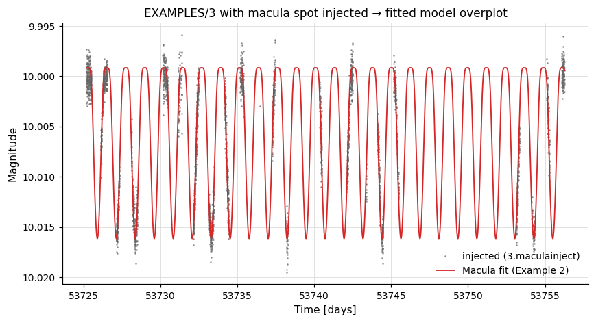
Example 2. Fit the Macula model to the simulated LC from Example 1 with the downhill-simplex optimiser. -LS first finds the rotation period, which then seeds Prot. Only Prot and istar are marked vary; the other parameters are held at their initial values. The fit is evaluated both at the observed times (omodel) and on a uniform grid for plotting (ocurve).
vartools -i EXAMPLES/OUTDIR1/3.maculainject \
    -stats t min \
    -LS 0.1 100 0.1 1 0 \
    -macula fit amoeba \
        Prot fixcolumn LS_Period_1_1 vary \
        istar fix 1.6 vary \
        kappa2 fix 0.0 \
        kappa4 fix 0.0 \
        c1 fix 0.2 c2 fix 0.1 c3 fix 0.0 c4 fix 0.0 \
        d1 fix 0.2 d2 fix 0.1 d3 fix 0.0 d4 fix 0.0 \
        blend fix 1.0 \
        Nspot 1 \
            Lambda0 fix 0.0 \
            Phi0 fix 1.2345 \
            alphamax fix 0.2 \
            fspot fix 0.1 \
            tmax fixcolumn STATS_t_MIN_0 \
            life fix 1000.0 \
            ingress fix 0.1 \
            egress fix 0.1 \
        omodel EXAMPLES/OUTDIR1 \
        ocurve EXAMPLES/OUTDIR1 \
    -oneline
The injected light curve from Example 1 with the Example 2 fitted-model curve overplotted:
-magadd
Add a constant offset to light curve magnitudes.
Syntax
Description
Add a scalar offset to every magnitude in the light curve. The offset can be a fixed constant, a per-LC value from the input list, a previously computed output statistic, or an analytic expression. This is also the canonical template extension included in the source tree to demonstrate how to write user-defined VARTOOLS extensions.
Python equivalent: magadd.
Parameters
| Source keyword | Description |
|---|---|
"fix" value |
Add the same constant to all light curves. |
"list" ["column" col] |
Read the offset per LC from the input list. |
"fixcolumn" col |
Take the offset from a previously computed output statistic. |
"expr" expr |
Evaluate an analytic expression per LC. |
Output columns: Magadd_addval_N (the value applied for that LC).
Examples
Example 1. Add a constant 0.5 mag to every observation of EXAMPLES/2. The two -rms calls before and after -magadd show that the mean magnitude shifts by 0.5 while the RMS is unchanged.