Period Finding / Signal Detection

This page documents the VARTOOLS commands for detecting and characterizing signals in light curves, both periodic (Lomb-Scargle, AoV, PDM, BLS, FTP, wavelets) and template-shaped transients (matched filter). Commands output peak periods or trial-centre times, significance, and signal-to-noise statistics to the output table; periodograms / matched-filter surfaces are optionally written to on-disk files.

---

-LS — Generalized Lomb-Scargle

Syntax

-LS
    < "var" minpvar | "expr" minpexpr | minp >
    < "var" maxpvar | "expr" maxpexpr | maxp >
    < "var" subsamplevar | "expr" subsampleexpr | subsample >
    Npeaks operiodogram [outdir] ["noGLS"]
    ["whiten"] ["clip" clip clipiter]
    ["fixperiodSNR" < "aov" | "ls" | "injectharm" | "fix" period
                    | "list" ["column" col]
                    | "fixcolumn" <colname | colnum> >]
    ["bootstrap" Nbootstrap] ["maskpoints" maskvar]

Description

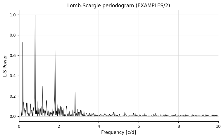
Perform a Generalized Lomb-Scargle (GLS) period search for sinusoidal signals. The search runs over frequencies from fmin = 1/maxp to fmax = 1/minp with a uniform frequency step Δf = subsample/T, where T is the time baseline. The GLS implementation of Zechmeister and Kürster (2009) allows a floating mean and heteroscedastic errors, unlike the traditional LS periodogram.

For each of the three search parameters (minp, maxp, subsample) you may either give a fixed value on the command line, use the "var" keyword followed by a variable name, or use the "expr" keyword to evaluate an analytic expression for each light curve.

Python equivalent: LS.

The statistic reported is:

LS = (chi0^2 - chi(f)^2) / chi0^2

where chi0^2 is χ² about the weighted mean and chi(f)^2 is χ² about the best-fit sinusoid at frequency f. For the traditional (non-generalized) periodogram, LS is the standard un-normalized Lomb-Scargle power.

Parameters

Parameter	Description
minp	Minimum period to search (days).
maxp	Maximum period to search (days).
subsample	Frequency oversampling factor. Typical value: 0.1 (one-tenth of the fundamental frequency resolution).
Npeaks	Number of highest peaks to find and report.
operiodogram	1 to write the periodogram to outdir/$basename.ls; 0 to skip.
outdir	Directory for periodogram files (required when operiodogram = 1).
"noGLS"	Compute the traditional (non-generalized) Lomb-Scargle periodogram.
"whiten"	After each peak, whiten the light curve at that period before searching for the next peak. The SNR for each peak is computed on the whitened periodogram.
"clip" clip clipiter	Sigma-clipping parameters for the mean/RMS calculation used in the SNR estimate. clip is the clipping factor; clipiter is 1 for iterative clipping (default: iterative 5σ).
"fixperiodSNR" ...	Also output log(FAP) and SNR at a specified period. Sources: "aov" (last -aov), "ls" (last -LS), "injectharm" (last -Injectharm), "fix" period, "list", or "fixcolumn".
"bootstrap" Nbootstrap	Estimate the FAP via bootstrap resampling (Nbootstrap simulations). Each simulation uses the observed times with magnitudes drawn randomly with replacement.
"maskpoints" maskvar	Exclude points with maskvar ≤ 0 from the periodogram calculation.

Output columns (per peak k, command index i)

Column	Description
LS_Period_k_i	Best period of peak k (days).
Log10_LS_Prob_k_i	Log₁₀ of the formal false alarm probability.
LS_SNR_k_i	Spectroscopic SNR: (LS - <LS>) / RMS(LS).

References

Cite Zechmeister & Kürster 2009, A&A, 496, 577 and Press et al. 1992 (Numerical Recipes) for the GLS periodogram. For the traditional LS periodogram also cite Lomb 1976, Scargle 1982, and Press & Rybicki 1989.

Examples

Example 1. Run the Lomb-Scargle period search on a single light curve, reporting the top 5 peaks, writing periodograms, applying whitening, and using iterative 5σ clipping for SNR.

vartools -i EXAMPLES/2 -oneline -ascii \
    -LS 0.1 10. 0.1 5 1 EXAMPLES/OUTDIR1 whiten clip 5. 1

Output:

LS_Period_1_0 = 1.23440877 (Log10_LS_Prob = -704.49194, LS_SNR = 126.52865)
LS_Period_2_0 = 0.54573861 (Log10_LS_Prob = -60.19769, LS_SNR = 12.22747)
LS_Period_3_0 = 0.55647766 (Log10_LS_Prob = -52.64556, LS_SNR = 9.46714)
LS_Period_4_0 = 0.25922584 (Log10_LS_Prob = -28.26507, LS_SNR = 7.42006)
LS_Period_5_0 = 0.50172744 (Log10_LS_Prob = -25.89142, LS_SNR = 8.63338)

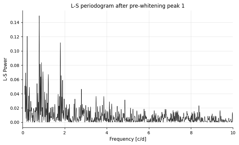
After pre-whitening peak 1 the periodogram looks like this — the dominant 1.234-day signal has been removed; subsequent peaks are now visible above the residual:

---

-aov — Phase-Binned Analysis of Variance

Syntax

-aov
    ["Nbin" < "var" Nbinvar | "expr" Nbinexpr | Nbin >]
    < "var" minpvar | "expr" minpexpr | minp >
    < "var" maxpvar | "expr" maxpexpr | maxp >
    < "var" subsamplevar | "expr" subsampleexpr | subsample >
    < "var" finetunevar | "expr" finetuneexpr | finetune >
    Npeaks operiodogram [outdir]
    ["whiten"] ["clip" clip clipiter] ["uselog"]
    ["fixperiodSNR" < "aov" | "ls" | "injectharm" | "fix" period
                    | "list" ["column" col]
                    | "fixcolumn" <colname | colnum> >]
    ["maskpoints" maskvar]

Description

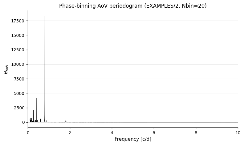
Perform an Analysis of Variance (AoV) period search using phase binning. For each trial frequency, the light curve is phase-folded and binned; the AoV statistic θ_aov measures how much variance is explained by the phase bins relative to the total variance. A high θ_aov indicates a good phase-coherent signal.

The initial search uses a frequency step of subsample/T. The top peaks are refined to a resolution of finetune/T.

Python equivalent: aov.

Parameters

Parameter	Description
"Nbin"	Number of phase bins (default: 8).
minp / maxp	Period search range (days). Accepts "var" or "expr" keywords.
subsample	Coarse frequency step factor.
finetune	Fine-tuning frequency step factor applied near peak periods.
Npeaks	Number of peaks to report.
operiodogram	1 to write period vs. θ_aov to outdir/$basename.aov.
"whiten"	Whiten the light curve at each peak before searching for the next one.
"clip" clip clipiter	Clipping parameters for the SNR calculation.
"uselog"	Output ln(θ_aov) SNR: (<-ln(θ_aov)> - ln(θ_aov)) / RMS(-ln(θ_aov)). Also outputs the mean and RMS of -ln(θ_aov).
"fixperiodSNR" ...	Output AoV statistic and SNR at a specified period. Syntax identical to -LS.
"maskpoints" maskvar	Exclude points with maskvar ≤ 0.

Output columns (per peak k, command index i)

Column	Description
Period_k_i	Best period of peak k (days).
AOV_k_i	θ_aov statistic.
AOV_SNR_k_i	Signal-to-noise ratio in the periodogram.
AOV_NEG_LOG_FAP_k_i	-ln(FAP) (formal false alarm probability).

References

Cite Schwarzenberg-Czerny 1989, MNRAS, 241, 153 and Devor 2005, ApJ, 628, 411.

Examples

Example 1. Run the phase-binning AoV period search on a light curve, using 20 phase bins, searching periods between 0.1 and 10.0 days, reporting the top 5 peaks with iterative 5σ clipping.

vartools -i EXAMPLES/2 -oneline -ascii \
    -aov Nbin 20 0.1 10. 0.1 0.01 5 1 EXAMPLES/OUTDIR1 whiten clip 5. 1

Output: Five detected periods with Period_1_0 = 1.23583047 (AOV_1_0 = 18330.55450, AOV_SNR, AOV_NEG_LN_FAP) through Period_5_0 = 0.12056969 (AOV_5_0 = 16.69317), with corresponding SNR and negative log FAP values for each.

---

-aov_harm — Multi-Harmonic Analysis of Variance

Syntax

-aov_harm
    < "var" Nharmvar | "expr" Nharmexpr | Nharm >
    < "var" minpvar | "expr" minpexpr | minp >
    < "var" maxpvar | "expr" maxpexpr | maxp >
    < "var" subsamplevar | "expr" subsampleexpr | subsample >
    < "var" finetunevar | "expr" finetuneexpr | finetune >
    Npeaks operiodogram [outdir]
    ["whiten"] ["clip" clip clipiter]
    ["fixperiodSNR" < "aov" | "ls" | "injectharm" | "fix" period
                    | "list" ["column" col]
                    | "fixcolumn" <colname | colnum> >]
    ["maskpoints" maskvar]

Description

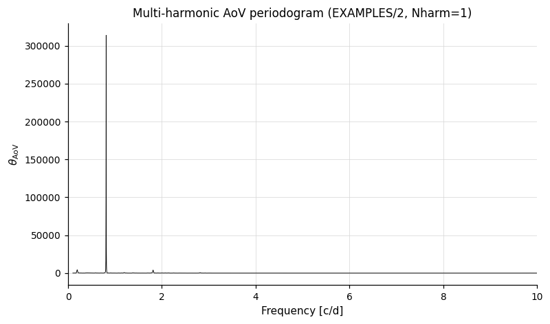
Perform an AoV period search fitting a multi-harmonic model instead of phase bins. The model signal has Nharm harmonics. If Nharm < 1, the number of harmonics is automatically varied to minimize the false alarm probability (accounting for the penalty for overfitting). All other parameters are identical to -aov.

Python equivalent: aov_harm.

Parameters

Parameter	Description
Nharm	Number of harmonics in the model signal (≥ 1). Set to 0 or negative to allow automatic selection. Accepts "var" or "expr" keywords.
All others	Same as -aov.

Output columns

Same structure as -aov with prefix AOV_HARM.

References

Cite Schwarzenberg-Czerny 1996, ApJ, 460, L107.

Examples

Example 1. Run the multi-harmonic AoV period search with 1 harmonic, searching periods between 0.1 and 10.0 days, reporting the top 2 peaks with whitening and iterative 5σ clipping.

vartools -i EXAMPLES/2 -oneline -ascii \
    -aov_harm 1 0.1 10. 0.1 0.01 2 1 EXAMPLES/OUTDIR1 whiten clip 5. 1

Output: Period values and AOV_HARM, SNR, and logarithmic FAP values for 2 identified peaks (1.23533969 days and 0.49981672 days).

---

-PDM — Phase Dispersion Minimization

Syntax

-PDM < "step" | "linterp" | "multicover" | "tophat" | "gauss" >
    ["Nbin" < "var" Nbinvar | "expr" Nbinexpr | Nbin >]
    ["Nc"   < "var" Ncvar   | "expr" Ncexpr   | Nc >]
    ["dphi" < "var" dphivar | "expr" dphiexpr | dphi >]
    < "var" minpvar | "expr" minpexpr | minp >
    < "var" maxpvar | "expr" maxpexpr | maxp >
    < "var" subsamplevar | "expr" subsampleexpr | subsample >
    < "var" finetunevar | "expr" finetuneexpr | finetune >
    Npeaks operiodogram [outdir]
    ["clip" clip clipiter] ["noerr"] ["whiten"]
    ["fixperiodSNR" < "aov" | "ls" | "pdm" | "injectharm" | "fix" period
                    | "list" ["column" col]
                    | "fixcolumn" <colname | colnum> >]
    ["bootstrap" Nboot] ["maskpoints" maskvar]

Description

Perform a Phase Dispersion Minimization (PDM) period search. For each trial frequency the light curve is phase-folded and a statistic θ ∈ [0, 1] measures the residual dispersion against a phase-fold model. A signal at the correct period produces θ near 0; pure noise yields θ near 1. The first argument selects one of five variants:

Variant	Model	Notes
step	Per-bin mean over Nbin fixed phase bins (Stellingwerf 1978).	Classic PDM.
linterp	Linear interpolation between adjacent bin means (cuvarbase default).	Smoother periodogram than step; less bin-edge sensitivity for the same Nbin.
multicover	Average of Nc phase-shifted Nb-bin sets (each shifted by 1/(Nb·Nc)).	Reduces bin-edge sensitivity at the cost of more computation. Schwarzenberg-Czerny 1997 explicitly notes that no analytic FAP exists for Nc > 1; the reported PDM_NEG_LN_FAP uses the single-cover Beta formula and should be treated as approximate.
tophat	Per-point weighted mean of phase-neighbours inside \|Δφ\| ≤ dphi.	Binless — no phase grid. Useful for sparse light curves where bin occupancy is irregular. Costs O(N²) per trial period.
gauss	Per-point weighted mean with Gaussian phase kernel of sigma dphi.	Smoother binless variant. Same O(N²) cost.

The initial search uses a frequency step of subsample/T. The top peaks are refined to a resolution of finetune/T. Defaults: Nbin = 8, Nc = 2 (for multicover), dphi = 0.05 (for tophat/gauss).

Python equivalent: PDM.

Parameters

Parameter	Description
variant	Required: one of step, linterp, multicover, tophat, gauss.
"Nbin"	Number of phase bins (per cover for multicover). Default 8. Rejected with tophat/gauss. Accepts "var"/"expr".
"Nc"	Number of phase-shifted bin sets, multicover only. Default 2. Accepts "var"/"expr".
"dphi"	Phase-window half-width (tophat) or kernel sigma (gauss). Default 0.05. Rejected with binned variants. Accepts "var"/"expr".
minp / maxp	Period search range (days). Accepts "var"/"expr".
subsample	Coarse frequency step factor. The coarse-grid frequency step is Δf = subsample / T, where T is the time-span of the light curve.
finetune	Fine-tuning frequency step factor applied near peak periods. The fine-tune step is Δf_fine = finetune / T.
Npeaks	Number of peaks to report.
operiodogram	1 to write period vs. θ to outdir/$basename.pdm. When whiten is set, the file gains one column per whitening cycle.
"clip" clip clipiter	σ-clipping factor and iterate-flag for the periodogram mean/RMS used in the SNR. Default 5σ iterative, matching -aov.
"noerr"	Use uniform point weights instead of 1/σ².
"whiten"	Subtract the step-bin phase model at each peak before searching for the next. Adds per-cycle Mean_PDM_Theta_k_N and RMS_PDM_Theta_k_N output columns; the periodogram dump gains one column per cycle.
"fixperiodSNR" ...	Report θ/SNR/FAP at a specified period in addition to the peak search. Sources: aov / ls / pdm (the most recent prior period-finder of that type), injectharm, fix period, list (with optional column N), or fixcolumn name.
"bootstrap" Nboot	Replace the analytic Schwarzenberg-Czerny FAP with an empirical FAP calibrated from Nboot shuffled-light-curve trials. Bootstrap can be used to calibrate the FAP; in practice it may be too slow for large analysis projects.
"maskpoints" maskvar	Exclude points where maskvar ≤ 0.

The trailing keyword block is parsed in a strict order matching the syntax shown above; mis-ordering or duplicating these keywords produces a command-syntax error.

Output columns (per peak k, command index N)

Column	Description
PDM_Period_k_N	Best period of peak k (days).
PDM_Theta_k_N	θ statistic (lower is better; 1 = random, 0 = perfectly coherent).
PDM_SNR_k_N	(θ_mean − θ_peak) / θ_rms using the (possibly clipped) periodogram noise estimate. A poor significance statistic for PDM — included for consistency with -aov; prefer PDM_NEG_LN_FAP_k_N for thresholding.
PDM_NEG_LN_FAP_k_N	−ln(FAP). Computed analytically from the Schwarzenberg-Czerny 1997 Beta((N−Nb)/2, (Nb−1)/2) distribution with an effective-trials-factor correction, or empirically from the bootstrap distribution when "bootstrap" is set. Rigorous for step under standard ANOVA assumptions; approximate for the other variants.
Mean_PDM_Theta_N / RMS_PDM_Theta_N	Periodogram mean and RMS used for the SNR (one set per command unless whiten is set, in which case the per-cycle pairs Mean_PDM_Theta_k_N / RMS_PDM_Theta_k_N are emitted instead).

When fixperiodSNR is set, four additional columns are appended: PDM_PeriodFix_N, PDM_Theta_PeriodFix_N, PDM_SNR_PeriodFix_N, PDM_NEG_LN_FAP_PeriodFix_N.

References

Cite Stellingwerf 1978, ApJ, 224, 953 and Schwarzenberg-Czerny 1997, ApJ, 489, 941. See also Zalian, Chadid & Stellingwerf 2014, MNRAS, 440, 68 for a modern restatement. The linterp variant follows the implementation in cuvarbase (package developed by John Hoffman; the linterp PDM contribution was written by Attila Bodi).

Examples

Example 1. Phase-binned PDM with linear interpolation between bin means, top 5 peaks, iterative 5σ clipping, periodogram dump.

vartools -i EXAMPLES/2 -oneline \
    -PDM linterp Nbin 20 0.1 10. 0.1 0.01 5 1 EXAMPLES/OUTDIR1 \
        clip 5. 1 whiten

Example 2. Multicover variant with 8 bins per cover and 4 phase-shifted covers — useful when bin-edge sensitivity dominates a step-PDM analysis.

vartools -i EXAMPLES/2 -oneline \
    -PDM multicover Nbin 8 Nc 4 0.1 10. 0.1 0.01 3 1 EXAMPLES/OUTDIR1

Example 3. Binless tophat variant on a narrower period range (binless variants cost O(N²) per trial frequency).

vartools -i EXAMPLES/2 -oneline \
    -PDM tophat dphi 0.05 0.5 2.0 0.5 0.05 2 1 EXAMPLES/OUTDIR1

Example 4. Bootstrap-calibrated empirical FAP (2000 trials, fixed RNG seed for reproducibility).

vartools -i EXAMPLES/2 -oneline -randseed 1 \
    -PDM linterp Nbin 8 0.1 10. 0.1 0.01 3 0 \
        bootstrap 2000

---

-FTP — Fast Template Periodogram

Syntax

-FTP < "file" template_file
     | "fitlc" lc_path
            < "ascii" t_col mag_col err_col
            | "fits"  t_colname mag_colname err_colname >
            Nharm period
     | "inline" Nharm
            < "var" c1var | "expr" c1expr | c1 >
            < "var" s1var | "expr" s1expr | s1 > ...
            (2*(Nharm+1) coefficient specs)
     | "filelist" ["column" colnum] >
    < "var" minpvar | "expr" minpexpr | minp >
    < "var" maxpvar | "expr" maxpexpr | maxp >
    < "var" subsamplevar | "expr" subsampleexpr | subsample >
    < "var" finetunevar | "expr" finetuneexpr | finetune >
    Npeaks operiodogram [outdir]
    ["clip" clip clipiter] ["noerr"] ["posamponly"] ["whiten"]
    ["fixperiodSNR" < "aov" | "ls" | "pdm" | "ftp" | "injectharm" | "fix" period
                    | "list" ["column" col]
                    | "fixcolumn" <colname | colnum> >]
    ["bootstrap" Nboot] ["maskpoints" maskvar]
    ["method" < "auto" | "brute" | "poly" | "verify" >]
    ["sums"   < "auto" | "direct" | "nfft" >]

Description

Perform a Fast Template Periodogram (FTP) search. FTP is a non-linear extension of the generalised Lomb-Scargle periodogram (Hoffman, VanderPlas, Hartman & Bakos 2021) that fits a known periodic template shape M(φ) = Σₙ₌₁..ₕ [cₙ cos(n φ) + sₙ sin(n φ)] at each trial period instead of a single sinusoid. The reported FTP_Power_k_N ∈ [0, 1] is the fraction of the centred chi-square variance explained by the best-fit template at the trial period; 1 = exact fit. FTP is most useful when the signal shape is known a priori — RR Lyrae and Cepheid templates, or any signal whose Fourier coefficients can be reliably pre-computed.

The first argument selects how the template is sourced:

Mode	Description
file	Read cₙ, sₙ directly from a two-column whitespace-separated text file. The file has H rows: column 1 is cₙ, column 2 is sₙ. H is inferred from the row count. Lines starting with # and blank lines are ignored.
fitlc	Build the template by fitting a Fourier series of total order Nharm + 1 to the light curve at lc_path at the fixed period. Format ascii takes 1-indexed column numbers (use err_col = 0 for an unweighted fit); fits takes column-name strings (use err_colname = "none" for an unweighted fit). The resulting template is mean-subtracted and amplitude-normalised so the half peak-to-peak of M(φ) is 1.
inline	Specify the 2*(Nharm + 1) coefficients c₁, s₁, c₂, s₂, … directly. Each slot is a literal float, a var keyword followed by a variable name, or an expr keyword followed by a quoted expression — var / expr forms evaluate per light curve, allowing the template to vary across LCs. No mean-subtraction or normalisation is applied.
filelist	Read each LC's template file path from a column of the -l input list. Without column N the next available column is used. Each LC's template is loaded just before its periodogram runs, so H can differ across the list. If an LC's template fails to load, that LC is skipped (sentinel-filled output) and the run continues.

Following the -harmonicfilter / -Injectharm convention, Nharm counts harmonics above the fundamental — so Nharm = 0 is a pure-fundamental (sinusoidal) template with H = 1, Nharm = 1 adds a 2nd harmonic for H = 2, and so on.

The initial search uses a frequency step of subsample/T; the top peaks are refined to a resolution of finetune/T. The default method = "auto" selects the polynomial fast path for H ≤ 2 and the brute-force grid scan otherwise — the polynomial path is faster only for very low harmonic counts (the per-frequency contraction cost scales as H⁴). The default sums = "auto" selects NFFT-batched summation when vartools was built with --with-nfft (roughly 4× faster than per-frequency direct loops at N = 10⁴), and falls back to direct otherwise.

For non-sinusoidal templates an amplitude θ₁ < 0 is not a phase shift — it corresponds to a flipped template, which generally does not match the input signal. By default the search reports the global maximum of the periodogram regardless of sign, with FTP_NegAmp_k_N = 1 flagging suspect peaks; pass "posamponly" to skip negative-amplitude solutions during the search.

By default the Beta distribution from GLS is used to estimate the false alarm probability (FAP) - this is not formally correct, but should have similar asymptotic behavior to the true FAP. Use "bootstrap" Nboot to enable an empirical-CDF FAP calibrated from Nboot shuffled-light-curve trials (mirrors -LS / -PDM bootstrap; with whiten the distribution is calibrated once from the original LC). For peaks more extreme than any trial a log-log polynomial extrapolation to the most-extreme 10% of the bootstrap distribution is used.

Python equivalent: FTP.

Parameters

Parameter	Description
template_source	Required: file, fitlc, inline, or filelist; selects which of the mode-specific sub-syntaxes is in effect.
template_file	file mode only: path to a two-column cₙ sₙ text file.
lc_path	fitlc mode only: path to the light curve from which the template is built.
ascii t_col mag_col err_col / fits t_colname mag_colname err_colname	fitlc mode only: format-specific column specifiers. err_col = 0 (ASCII) or err_colname = "none"/"" (FITS) requests an unweighted fit.
Nharm	fitlc / inline modes: harmonics above the fundamental. Total template harmonic count is Nharm + 1.
period	fitlc mode only: fixed period at which the template Fourier series is fit (literal float — var / expr are not accepted for this slot).
c1 s1 c2 s2 …	inline mode: 2*(Nharm + 1) coefficient specs in alternating c/s order. Each spec is a literal float, "var" name, or "expr" text.
column colnum	filelist mode only: 1-indexed column of the -l input list holding each LC's template path. Optional; the next available column is used when omitted.
minp / maxp	Period search range (days). Accepts "var"/"expr".
subsample	Coarse frequency step factor (Δf = subsample / T).
finetune	Fine-tune frequency step factor near peak periods (Δf_fine = finetune / T).
Npeaks	Number of peaks to report.
operiodogram	1 to write period vs. FTP power to outdir/$basename.ftp. With whiten, one column per whitening cycle.
"clip" clip clipiter	σ-clipping factor and iterate-flag for the SNR noise estimate. Default 5σ iterative, matching -aov / -PDM.
"noerr"	Use uniform point weights instead of 1/σ².
"posamponly"	Skip negative-amplitude solutions during the search — the periodogram becomes the best positive-amplitude fit at each frequency.
"whiten"	After each peak, subtract θ₁ · M(ω t − θ₂) + θ₃ from the LC and recompute the periodogram for the next peak. Adds per-cycle Mean_FTP_Power_k_N / RMS_FTP_Power_k_N columns (one pair per peak instead of the per-LC pair).
"fixperiodSNR" …	Additionally report FTP power / SNR / θ₂ / NegAmp at a specified period. Sources: aov / ls / pdm / ftp (the most recent prior period-finder of that type), injectharm, fix period, list (with optional column N), or fixcolumn name. Evaluation is against the original light curve even when whiten is set.
"bootstrap" Nboot	Enable empirical-CDF FAP via Nboot shuffled-LC trials.
"maskpoints" maskvar	Exclude points where maskvar ≤ 0.
"method" mode	Per-frequency optimisation: auto (default; poly for H ≤ 2, brute otherwise), brute (720-sample θ₂ scan + golden refinement; correct to ~1e-12), poly (root-finding via the Hoffman et al. polynomial), or verify (run both methods and emit a per-LC stderr comparison summary; returns the brute result).
"sums" mode	Per-LC summation strategy: auto (NFFT if built with --with-nfft, else direct), direct, or nfft.

The trailing keyword block is parsed in a strict order matching the syntax above; mis-ordering or duplicating these keywords produces a command-syntax error.

Output columns (per peak k, command index N)

Column	Description
FTP_Period_k_N	Best period of peak k (days).
FTP_Power_k_N	FTP power statistic ∈ [0, 1]; higher is better, 1 = exact template fit.
FTP_SNR_k_N	(P_peak − P_mean) / P_rms over the clipped periodogram.
FTP_NegAmp_k_N	1 if the best fit at the peak had θ₁ < 0 (flipped template — generally not a real signal for non-symmetric M(φ)); 0 otherwise.
FTP_Theta_k_N	Best-fit phase shift θ₂ in radians.
Mean_FTP_Power_N / RMS_FTP_Power_N	Periodogram mean and RMS used for the SNR (one set per command unless whiten is set, in which case per-cycle Mean_FTP_Power_k_N / RMS_FTP_Power_k_N are emitted instead).
FTP_NEG_LN_FAP_k_N	−ln(FAP). Estimated from the GLS Beta distribution by default. When bootstrap is set: read from the empirical CDF, or from a log-log extrapolation to the most-extreme 10% of the bootstrap distribution when the peak is more extreme than any trial.

When fixperiodSNR is set, five additional columns are appended: FTP_PeriodFix_N, FTP_Power_PeriodFix_N, FTP_SNR_PeriodFix_N, FTP_NegAmp_PeriodFix_N, FTP_Theta_PeriodFix_N, FTP_NEG_LN_FAP_PeriodFix_N.

References

Cite Hoffman, J., VanderPlas, J., Hartman, J. D., & Bakos, G. A. 2021, arXiv:2101.12348. The reference Python implementation is at PrincetonUniversity/FastTemplatePeriodogram (package developed by John Hoffman).

Examples

Example 1. File-mode pure-cosine (H = 1) template — the degenerate Lomb-Scargle-like case, useful for showing the output column structure.

vartools -i EXAMPLES/2 -oneline \
    -FTP file EXAMPLES/2.ftptemplate 0.1 10. 0.1 0.01 3 1 EXAMPLES/OUTDIR1

Example 2. Build a 6-harmonic template by fitting a Fourier series to the light curve at its known period, then search the same LC with iterative whitening between peaks.

vartools -i EXAMPLES/2 -oneline \
    -FTP fitlc EXAMPLES/2 ascii 1 2 3 5 1.235 \
         0.1 10. 0.1 0.01 3 0 \
         clip 5. 1 whiten

Example 3. Inline-specified template plus bootstrap FAP and a fixed-period evaluation.

vartools -i EXAMPLES/2 -oneline -randseed 1 \
    -FTP inline 1 1.0 0.0 0.3 0.0 \
         0.1 10. 0.1 0.01 2 0 \
         fixperiodSNR fix 1.235 bootstrap 500

Example 4. Per-LC template paths read from a column of the input list (-l).

vartools -l EXAMPLES/lc_list_ftp -header \
    -FTP filelist column 2 0.1 2.0 0.1 0.01 2 0

---

-matchedfilter — Inverse-Variance Matched Filter

Syntax

-matchedfilter "template"
    < "exp"       < "var" v | "expr" e | tau >
    | "doubleexp" < "var" v | "expr" e | tau_rise >
                  < "var" v | "expr" e | tau_decay >
    | "flare"     < "var" v | "expr" e | tfwhm >
    | "gauss"     < "var" v | "expr" e | sigma >
    | "box"       < "var" v | "expr" e | width >
    | "triangle"  < "var" v | "expr" e | width >
    | "trap"      < "var" v | "expr" e | rise >
                  < "var" v | "expr" e | flat >
                  < "var" v | "expr" e | fall >
    | "file"      template_file
    | "expr"      ["varname" name] "<expression>" >
    < "var" v | "expr" e | support_halfwidth >
    "mode" < "window" | "nfft" >
    "signs" < "both" | "positive" | "negative" >
    Npeaks omatchfile [outdir]
    ["min_separation" < "var" v | "expr" e | sep >]
    ["whiten"]
    ["maskpoints" maskvar]

Description

Run an inverse-variance matched filter over the light curve to detect template-shaped transients or features (flares, transits, eclipses, bumps). Unlike the periodogram commands above, the matched filter does not assume periodicity; it scans the LC for single-shot occurrences of a template-shaped feature. At each trial centre τ (one of the LC's own time points) the algorithm fits a scaled, time-shifted template g(t − τ) plus a local constant offset c to the data within the support window:

\[y_i \sim a \cdot g(t_i - \tau) + c + \text{noise}_i, \quad w_i = 1/\sigma_i^2\]

The offset c is a nuisance parameter that absorbs the LC's local baseline, so the absolute magnitude of the LC does not have to be pre-subtracted; the reported amplitude â is the perturbation amplitude in light-curve units at the peak. The best-fit amplitude and signed SNR are

\[\hat{a}(\tau) = \frac{\text{Cov}_w(y, g)}{\text{Var}_w(g)}, \quad \text{SNR}(\tau) = \hat{a}(\tau) \cdot \sqrt{\sum_i w_i (g_i - \langle g \rangle_w)^2}\]

taken over points with |t_i − τ| ≤ support_halfwidth. The SNR is signed: positive for matches that share the template's orientation, negative for inverted matches (e.g. detecting a transit with a positive box template gives a strongly-negative SNR). The matched filter is scale-invariant in g, so the named templates are normalised to peak amplitude 1.

The first argument selects how the template is sourced:

Mode	Description
exp	Single-decay exponential: g(s) = exp(−s/tau) for s ≥ 0, else 0. Parameter tau is the decay timescale.
doubleexp	Rise-then-decay profile (1 − exp(−s/tau_rise))·exp(−s/tau_decay) for s ≥ 0, normalised so the peak amplitude is 1.
flare	Davenport+2014 empirical M-dwarf flare template. Parameter tfwhm is the rise full-width-at-half-maximum.
gauss	Gaussian: g(s) = exp(−s²/(2 sigma²)).
box	Box: g(s) = 1 for |s| ≤ width/2, else 0.
triangle	Symmetric V at s = 0: g(s) = 1 − 2|s|/width for |s| ≤ width/2, else 0.
trap	Trapezoid: linear rise of duration rise, flat top of duration flat, linear fall of duration fall. Centred in s ∈ ±(rise + flat + fall)/2.
file	Read the template from a 2-column whitespace-separated ASCII file (column 1 = template-relative time s, column 2 = amplitude g(s)). Lines starting with # are skipped. Rows are sorted by t and exact-duplicate t values are dropped at load time. Linear interpolation between rows.
expr	Define the template analytically. The expression is evaluated per data point with a stump variable bound to the template-relative time s = t_i − τ within the support window. The stump variable is named "s" by default; pass "varname" NAME before the expression to use a different name. The expression may reference the stump variable, per-star scalars, and constants; light-curve-vector references are rejected at parse time.

In all cases the support_halfwidth argument is an outer truncation window: g(s) is zero for |s| > support_halfwidth regardless of the template's intrinsic shape.

The required mode keyword selects the algorithm:

Mode	Description
window	Exact for any time sampling, supports heteroscedastic σ. Trial centres are the LC's own (sorted) time points; two cursors sweep forward through the data to find each support window. Cost: O(N · n_window) where n_window is the average number of data points falling within ±support_halfwidth of each trial.
nfft	NFFT-batched evaluation (requires vartools built --with-nfft). Two adjoint NFFTs over the data nodes plus five forward NFFTs against three pre-FFT'd kernels (the support indicator, the template, and the template squared). Cost: O(N_nfft · log(N_nfft) + N). Assumes homoscedastic σ (median); sharp-edged templates (box, triangle, trap) develop a few-percent spectral-leakage artefact near the support boundary. Prefer mode window for the cleanest semantics when sharp edges or per-point σ matter.

The required signs keyword sets the polarity filter applied to peak ranking and the per-LC noise estimate: positive for bumps that match the template orientation, negative for inverted matches, both to rank by |SNR|.

Npeaks distinct peaks are found by iteratively picking the most significant remaining trial and masking a ±min_separation window around its τ. Default min_separation equals support_halfwidth. When whiten is set, the search additionally subtracts â · g(t − τ_k) from a working copy of the LC between peaks; the original LC is restored on return.

Python equivalent: MatchedFilter.

Parameters

Parameter	Description
template	One of exp, doubleexp, flare, gauss, box, triangle, trap, file, expr. Selects the template-source mode.
tau / tau_rise / tau_decay / tfwhm / sigma / width / rise / flat / fall	Template-specific scalar parameter(s). Each accepts the standard <"var" v \| "expr" e \| val> per-LC pattern.
template_file	file mode only: path to a 2-column ASCII file.
varname NAME	expr mode only: name of the time-relative variable in the expression. Default s.
<expression>	expr mode only: vartools-syntax analytic expression for g(s).
support_halfwidth	Outer truncation half-width. Accepts var / expr.
mode	window (exact, heteroscedastic) or nfft (NFFT-batched, homoscedastic).
signs	both, positive, or negative.
Npeaks	Number of peaks to report.
omatchfile	1 to write the (t, SNR, amplitude) surface to outdir/$basename.mf; 0 to suppress.
"min_separation" sep	Mask half-width around each peak. Default = support_halfwidth.
"whiten"	Iteratively subtract â · g(t − τ_k) from a working copy of the LC between peaks.
"maskpoints" maskvar	Optional. Exclude points where maskvar ≤ 1e-7.

The trailing keyword block is parsed in a strict order matching the syntax above.

Output columns (per peak k, command index N)

Column	Description
MatchedFilter_Time_k_N	Trial centre τ of the k-th peak.
MatchedFilter_SNR_k_N	Signed SNR at the peak.
MatchedFilter_Amplitude_k_N	Best-fit amplitude â at the peak, in light-curve units.
MatchedFilter_Mean_SNR_N / MatchedFilter_RMS_SNR_N	Mean and RMS of SNR(τ) over the sign-filtered trial grid.

References

Cite Davenport, J. R. A., Hawley, S. L., Hebb, L. et al. 2014, ApJ, 797, 122 when using the flare named-template kind. The matched-filter formulation itself is standard; Turin, G. L. 1960, IRE Transactions on Information Theory, IT-6, 311 ("An introduction to matched filters") is the canonical reference.

Examples

Example 1. Gaussian template, smooth-feature search.

vartools -i EXAMPLES/2 -oneline \
    -matchedfilter template gauss 0.5 2.0 mode window signs both 3 0

Example 2. Box template recovering an injected transit. signs negative keeps only inverted (dip) matches.

vartools -i EXAMPLES/3.transit -oneline \
    -matchedfilter template box 0.083 0.5 mode window signs negative 1 0

Example 3. Analytic exponential-decay template for flare-shaped events, with min_separation and pre-whitening between peaks.

vartools -i EXAMPLES/2 -oneline \
    -matchedfilter template expr "exp(-s/0.005) * (s>0)" 0.02 \
        mode window signs negative 5 0 min_separation 0.05 whiten

---

-BLS — Box-fitting Least Squares

Syntax

-BLS
    < "r" < "var" rminvar | "expr" rminexpr | rmin >
              < "var" rmaxvar | "expr" rmaxexpr | rmax > |
      "q" < "var" qminvar | "expr" qminexpr | qmin >
          < "var" qmaxvar | "expr" qmaxexpr | qmax > |
      "density" < "var" rhovar | ... | rho >
                < "var" minexpdurfracvar | ... | minexpdurfrac >
                < "var" maxexpdurfracvar | ... | maxexpdurfrac > >
    < "var" minpervar | "expr" minperexpr | minper >
    < "var" maxpervar | "expr" maxperexpr | maxper >
    < "nf" < ... | nfreq > |
      "df" < ... | dfreq > |
      "optimal" < ... | subsample > >
    < "var" nbinsvar | "expr" nbinsexpr | nbins >
    timezone Npeak outperiodogram [outdir] omodel [modeloutdir]
    correctlc ["extraparams"] ["fittrap"] ["nobinnedrms"]
    ["ophcurve" outdir phmin phmax phstep]
    ["ojdcurve" outdir jdstep]
    ["stepP" | "steplogP"]
    ["adjust-qmin-by-mindt" ["reduce-nbins"]]
    ["reportharmonics"]
    ["mergepeakdf" < "transit" mult | factor >]
    ["maskpoints" maskvar]

Description

Run the Box-Least Squares (BLS) transit search algorithm (Kovács, Zucker & Mazeh 2002). BLS searches for periodic box-shaped (trapezoidal) dips consistent with a transiting companion. The search is performed over a grid of trial periods and phase bins.

Python equivalent: BLS.

Three ways to specify the allowed range of transit durations:

• "q" qmin qmax — minimum and maximum fractional transit duration (fraction of the orbit spent in transit).
• "r" rmin rmax — minimum and maximum stellar radius in solar radii. The q range for each period is derived from q = 0.076·R^(2/3)·P^(-2/3).
• "density" rho minexpdurfrac maxexpdurfrac — stellar density (g/cm³) with minimum and maximum fractions of the expected circular-orbit transit duration.

Parameters

Parameter	Description
minper / maxper	Period search range in days.
"nf" nfreq	Total number of trial frequencies. Rule of thumb: nfreq ≈ T · (fmax - fmin) / (0.25·qmin).
"df" dfreq	Explicit frequency step size.
"optimal" subsample	Use Ofir (2014) optimal frequency spacing (requires "density" mode).
nbins	Number of phase bins (≥ 2/qmin).
timezone	Hours to add to UTC to obtain local time; used to compute the fraction of Δχ² from a single night.
Npeak	Number of peaks to find and report.
outperiodogram	1 to output the BLS spectrum (SN vs. period) to outdir/$basename.bls.
omodel	1 to output the best-fit box model to modeloutdir/$basename.bls.model.
correctlc	1 to subtract the transit model before passing to the next command.
"extraparams"	Include additional false-positive diagnostic parameters in the output.
"fittrap"	Fit a trapezoidal transit at each BLS peak. Adds qingress (fraction of transit duration in ingress) and OOTmag to output.
"nobinnedrms"	Compute BLS_SN without binned RMS (faster, but SN is suppressed for high-significance peaks).
"ophcurve" outdir phmin phmax phstep	Output a model phase curve to outdir/$basename.bls.phcurve.
"ojdcurve" outdir jdstep	Output a model light curve (JD space) to outdir/$basename.bls.jdcurve.
"stepP" / "steplogP"	Sample the BLS spectrum at uniform P or log(P) steps instead of uniform frequency steps.
"adjust-qmin-by-mindt"	Adaptively increase qmin at each frequency to max(qmin, mindt·f).
"reduce-nbins"	(With adjust-qmin-by-mindt) adaptively reduce nbins at each frequency.
"reportharmonics"	Report period harmonics even if a higher-power peak at a multiple of that frequency exists.
"mergepeakdf" < "transit" mult \| factor >	Set the frequency resolution Df used to decide whether two spectrum peaks are the same detection. By default Df = 1/T (the Rayleigh resolution, T = time baseline), which is appropriate for a sinusoid but tends to over-merge transit peaks (a box transit of fractional width q is resolved on the finer scale q/T). "transit" mult sets Df = mult·q/T using the per-candidate fitted transit width q (a mult of order a few is recommended); a bare number sets Df = factor/T (mergepeakdf 1.0 reproduces the default).
"maskpoints" maskvar	Exclude points with maskvar ≤ 0 from the BLS spectrum.

Output columns (per peak k, command index i)

Column	Description
BLS_Period_k_i	Best period of peak k (days).
BLS_Tc_k_i	Mid-transit epoch.
BLS_SN_k_i	Signal-to-noise ratio in the BLS spectrum.
BLS_SR_k_i	BLS spectral residual.
BLS_SDE_k_i	Signal detection efficiency.
BLS_Depth_k_i	Transit depth (magnitudes).
BLS_Qtran_k_i	Fractional transit duration q.
BLS_deltaChi2_k_i	Δχ² of the best-fit transit.
BLS_SignaltoPinknoise_k_i	Signal-to-pink-noise ratio.
BLS_Ntransits_k_i	Number of observed transits.
BLS_Npointsintransit_k_i	Points within the transit window.
BLS_fraconenight_k_i	Fraction of Δχ² from a single night.
BLS_Rednoise_k_i	Estimated red noise level.
BLS_Whitenoise_k_i	Estimated white noise level.

When "fittrap" is given, BLS_Qingress_k_i and BLS_OOTmag_k_i are also included.

References

Cite Kovács, Zucker & Mazeh 2002, A&A, 391, 369. For the optimal frequency sampling cite Ofir 2014, A&A, 561, A138.

Examples

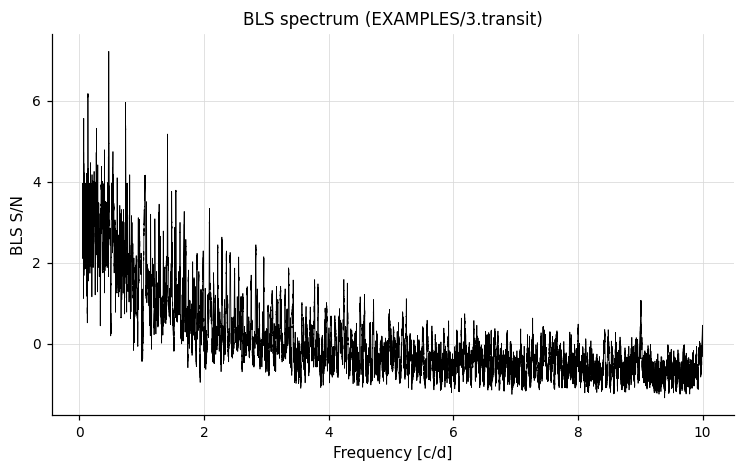
Example 1. Apply the BLS transit search to a light curve with an injected transit, scanning fractional durations 0.01–0.1, searching periods 0.1–20.0 days with 100,000 frequencies and 200 phase bins, fitting a trapezoid model and outputting a phase curve.

vartools -i EXAMPLES/3.transit -ascii -oneline \
    -BLS q 0.01 0.1 0.1 20.0 100000 200 0 1 \
        1 EXAMPLES/OUTDIR1/ 1 EXAMPLES/OUTDIR1/ 0 fittrap \
        nobinnedrms ophcurve EXAMPLES/OUTDIR1/ -0.1 1.1 0.001

Output:

Name                         = EXAMPLES/3.transit
BLS_Period_1_0               =     2.12334706
BLS_Tc_1_0                   = 53727.297293937358
BLS_SN_1_0                   =   7.26127
BLS_SR_1_0                   =   0.00238
BLS_SDE_1_0                  =   6.34195
BLS_Depth_1_0                =   0.01220
BLS_Qtran_1_0                =   0.03576
BLS_Qingress_1_0             =   0.19618
BLS_OOTmag_1_0               =  10.16686
BLS_i1_1_0                   =   0.98213
BLS_i2_1_0                   =   1.01790
BLS_deltaChi2_1_0            = -24217.21939
BLS_fraconenight_1_0         =   0.43155
BLS_Npointsintransit_1_0     =   165
BLS_Ntransits_1_0            =     4
BLS_Npointsbeforetransit_1_0 =   127
BLS_Npointsaftertransit_1_0  =   143
BLS_Rednoise_1_0             =   0.00151
BLS_Whitenoise_1_0           =   0.00489
BLS_SignaltoPinknoise_1_0    =  14.38935
BLS_Period_invtransit_0      =     1.14594782
BLS_deltaChi2_invtransit_0   = -3301.69183
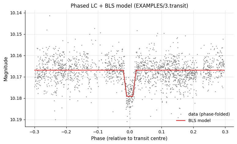
BLS_MeanMag_0                =  10.16740

The output *.bls.model file contains the phased data and the best-fit trapezoidal transit model — together they look like:

---

-BLSFixPer — BLS at a Fixed Period

Syntax

-BLSFixPer
    < "aov" | "ls" | "list" ["column" col]
      | "fix" period | "fixcolumn" <colname | colnum>
      | "expr" expr >
    < "r" rmin rmax | "q" qmin qmax >
    nbins timezone omodel [model_outdir] correctlc ["fittrap"]
    ["maskpoints" maskvar]

Description

Run BLS at a single fixed period, searching only for the most transit-like signal at that period. Useful as a second pass after a full BLS or LS period search.

Python equivalent: BLSFixPer.

Parameters

Parameter	Description
Period source	"aov" (last -aov), "ls" (last -LS), "list", "fix" period, "fixcolumn", or "expr".
"r" rmin rmax / "q" qmin qmax	Transit duration range (stellar radius bounds or fractional duration bounds).
nbins	Number of phase bins.
timezone	UTC offset for single-night fraction calculation.
omodel	1 to output the model to model_outdir (suffix: .blsfixper.model).
correctlc	1 to subtract the model from the light curve.
"fittrap"	Fit a trapezoid transit at the BLS peak.
"maskpoints" maskvar	Exclude points with maskvar ≤ 0.

References

Cite Kovács, Zucker & Mazeh 2002, A&A, 391, 369.

Examples

Example 1. Fit a box-shaped (with trapezoid fitting) transit model at a fixed period of 2.12345 days, scanning fractional durations 0.01–0.1 with 200 phase bins, and compute RMS before and after subtracting the transit.

vartools -i EXAMPLES/3.transit -ascii -oneline \
    -rms \
    -BLSFixPer fix 2.12345 q 0.01 0.1 200 0 0 1 fittrap \
    -rms

Output:

Name                             = EXAMPLES/3.transit
Mean_Mag_0                       =  10.16727
RMS_0                            =   0.00542
Expected_RMS_0                   =   0.00104
Npoints_0                        =  3417
BLSFixPer_Period_1               =  2.12345000
BLSFixPer_Tc_1                   = 53727.29676321477
BLSFixPer_SR_1                   =   0.00238
BLSFixPer_Depth_1                =   0.01189
BLSFixPer_Qtran_1                =   0.03626
BLSFixPer_Qingress_1             =   0.20623
BLSFixPer_OOTmag_1               =  10.16687
BLSFixPer_i1_1                   =   0.98158
BLSFixPer_i2_1                   =   1.01785
BLSFixPer_deltaChi2_1            = -24228.56603
BLSFixPer_fraconenight_1         =   0.43366
BLSFixPer_Npointsintransit_1     =   166
BLSFixPer_Ntransits_1            =     4
BLSFixPer_Npointsbeforetransit_1 =   129
BLSFixPer_Npointsaftertransit_1  =   144
BLSFixPer_Rednoise_1             =   0.00151
BLSFixPer_Whitenoise_1           =   0.00489
BLSFixPer_SignaltoPinknoise_1    =  14.08946
BLSFixPer_deltaChi2_invtransit_1 = -2934.30109
BLSFixPer_MeanMag_1              =  10.16740
Mean_Mag_2                       =  10.16678
RMS_2                            =   0.00489
Expected_RMS_2                   =   0.00104
Npoints_2                        =  3417

---

-BLSFixDurTc — BLS with Fixed Transit Duration and Epoch

Syntax

-BLSFixDurTc
    <"duration" <"fix" dur | "var" varname | "expr" expression
        | "fixcolumn" <colname | colnum>
        | "list" ["column" col]>>
    <"Tc" <"fix" Tc | "var" varname | "expr" expression
        | "fixcolumn" <colname | colnum>
        | "list" ["column" col]>>
    ["fixdepth" <"fix" depth | "var" varname | "expr" expression
        | "fixcolumn" <colname | colnum>
        | "list" ["column" col]>
        ["qgress" <"fix" qgress | "var" varname | "expr" expression
            | "fixcolumn" <colname | colnum>
            | "list" ["column" col]>]]
    <"var" minpvar | "expr" minpexpr | minper>
    <"var" maxpvar | "expr" maxpexpr | maxper>
    <"var" nfvar | "expr" nfexpr | nfreq> timezone
    Npeak outperiodogram [outdir] omodel [model_outdir]
    correctlc ["fittrap"]
    ["ophcurve" outdir phmin phmax phstep]
    ["ojdcurve" outdir jdstep]
    ["mergepeakdf" < "transit" mult | factor >]
    ["maskpoints" maskvar]

Description

Run BLS with the transit duration and a reference epoch fixed. The period is still searched over a grid from minper to maxper. Optionally the transit depth and ingress fraction (qgress) can be fixed as well. For qgress: 0 = box-shaped transit; 0.5 = V-shaped (grazing) transit.

Python equivalent: BLSFixDurTc.

Parameters

Parameter	Description
"duration"	Transit duration. Source: "fix" (command line), "fixcolumn", or "list".
"Tc"	Reference transit epoch. Same source options as "duration".
"fixdepth"	Optionally fix the transit depth.
"qgress"	Optionally fix the ingress fraction.
minper / maxper / nfreq	Period range and number of trial frequencies.
All others	Same as -BLS.

Examples

Example 1. Run a BLS search on EXAMPLES/3.transit fixing the transit duration to 0.076996297 days and the transit epoch to 53727.29676321477. Search periods between 0.1 and 20 days using 100,000 frequency steps. The time-zone is set to 0 (only affects the BLSFixPer_fraconenight statistic). The periodogram and model are not output, but the best-fit model is subtracted from the light curve before passing it to the next command. The fittrap keyword fits a trapezoidal transit. The two -rms calls show how subtracting the BLS model reduces the scatter.

vartools -i EXAMPLES/3.transit -oneline \
    -rms \
    -BLSFixDurTc duration fix 0.076996297 \
        Tc fix 53727.29676321477 0.1 20. 100000 \
        0 1 0 0 1 fittrap \
    -rms

References

Cite Kovács, Zucker & Mazeh 2002, A&A, 391, 369.

---

-BLSFixPerDurTc — BLS with Fixed Period, Duration, and Epoch

Syntax

-BLSFixPerDurTc
    <"period" <"fix" per | "var" varname | "expr" expression
        | "fixcolumn" <colname | colnum>
        | "list" ["column" col]>>
    <"duration" <"fix" dur | "var" varname | "expr" expression
        | "fixcolumn" <colname | colnum>
        | "list" ["column" col]>>
    <"Tc" <"fix" Tc | "var" varname | "expr" expression
        | "fixcolumn" <colname | colnum>
        | "list" ["column" col]>>
    ["fixdepth" <"fix" depth | "var" varname | "expr" expression
        | "fixcolumn" <colname | colnum>
        | "list" ["column" col]>
        ["qgress" <"fix" qgress | "var" varname | "expr" expression
            | "fixcolumn" <colname | colnum>
            | "list" ["column" col]>]]
    timezone omodel [model_outdir]
    correctlc ["fittrap"]
    ["ophcurve" outdir phmin phmax phstep]
    ["ojdcurve" outdir jdstep] ["maskpoints" maskvar]

Description

Run BLS with the period, transit duration, and reference epoch all fixed. Only the phase of the transit (within a single period) is searched. All options are similar to -BLSFixDurTc, except the period is also specified.

Python equivalent: BLSFixPerDurTc.

Examples

Example 1. Fit a box-shaped transit to EXAMPLES/3.transit at a fixed period of 2.12345 days, with the duration fixed at 0.076996297 days and the transit epoch at 53727.29676321477. The model is subtracted from the light curve and passed to the next command. The fittrap keyword fits a trapezoidal transit. The two -rms calls show how subtracting the BLS model reduces the scatter.

vartools -i EXAMPLES/3.transit -oneline \
    -rms \
    -BLSFixPerDurTc period fix 2.12345 \
        duration fix 0.076996297 \
        Tc fix 53727.29676321477 \
        0 0 1 fittrap \
    -rms

References

Cite Kovács, Zucker & Mazeh 2002, A&A, 391, 369.

---

-dftclean — DFT Power Spectrum + CLEAN

Syntax

-dftclean <"var" nbvar | "expr" nbexpr | nbeam>
    ["maxfreq" <"var" mfvar | "expr" mfexpr | maxf>]
    ["outdspec" dspec_outdir]
    ["finddirtypeaks" Npeaks ["clip" <"var" cvar | "expr" cexpr | clip>
    clipiter]]
    ["outwfunc" wfunc_outdir]
    ["clean" <"var" gvar | "expr" gexpr | gain> <"var" snvar | "expr" snexpr |
    SNlimit>
        ["outcbeam" cbeam_outdir]
    ["outcspec" cspec_outdir]
    ["findcleanpeaks" Npeaks ["clip" <"var" cvar | "expr" cexpr | clip>
    clipiter]]]
    ["useampspec"] ["verboseout"] ["maskpoints" maskvar]

Description

Compute the Discrete Fourier Transform (DFT) power spectrum of the light curve using the FDFT algorithm (Kurtz 1985) and optionally deconvolve it with the CLEAN algorithm (Roberts, Lehar & Dreher 1987) to remove aliasing due to the window function.

Python equivalent: dftclean.

Parameters

Parameter	Description
nbeam	Number of frequency samples per 1/T frequency element (T = light curve baseline). Controls the spectral resolution.
"maxfreq" maxf	Maximum frequency (cycles/day). Default: 1 / (2 · min_time_separation) (Nyquist).
"outdspec" dspec_outdir	Write the dirty (uncleaned) power spectrum to dspec_outdir/$basename.dftclean.dspec.
"finddirtypeaks" Npeaks	Find the top Npeaks peaks in the dirty spectrum.
"outwfunc" wfunc_outdir	Write the window function to wfunc_outdir/$basename.dftclean.wfunc.
"clean" gain SNlimit	Apply the CLEAN algorithm. gain ∈ [0.1, 1.0] (smaller = slower convergence, more thorough); iterations continue until the highest remaining peak is below SNlimit × noise.
"outcbeam" cbeam_outdir	Write the clean beam to cbeam_outdir/$basename.dftclean.cbeam.
"outcspec" cspec_outdir	Write the clean power spectrum to cspec_outdir/$basename.dftclean.cspec.
"findcleanpeaks" Npeaks	Find the top Npeaks peaks in the clean spectrum.
"clip" clip clipiter	Clipping parameters for peak SNR calculation (default: iterative 5σ).
"useampspec"	Compute SNR on the amplitude spectrum instead of the power spectrum.
"verboseout"	Include the mean and standard deviation of the spectrum before and after clipping in the output.
"maskpoints" maskvar	Exclude points with maskvar ≤ 0.

References

Cite Kurtz 1985, MNRAS, 213, 773 for the FDFT algorithm. Cite Roberts, Lehar & Dreher 1987, AJ, 93, 968 for the CLEAN algorithm.

Examples

Example 1. Compute the DFT power spectrum of a light curve up to 10 cycles/day, find the top dirty-spectrum peak using iterative 5σ clipping.

vartools -i EXAMPLES/2 -oneline -ascii \
    -dftclean 4 maxfreq 10. outdspec EXAMPLES/OUTDIR1 \
        finddirtypeaks 1 clip 5. 1

Output:

Name                         = EXAMPLES/2
DFTCLEAN_DSPEC_PEAK_FREQ_0_0 =     0.81189711
DFTCLEAN_DSPEC_PEAK_POW_0_0  = 0.000687634
DFTCLEAN_DSPEC_PEAK_SNR_0_0  =   59.8532

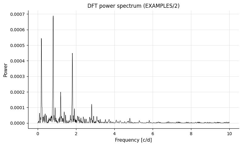
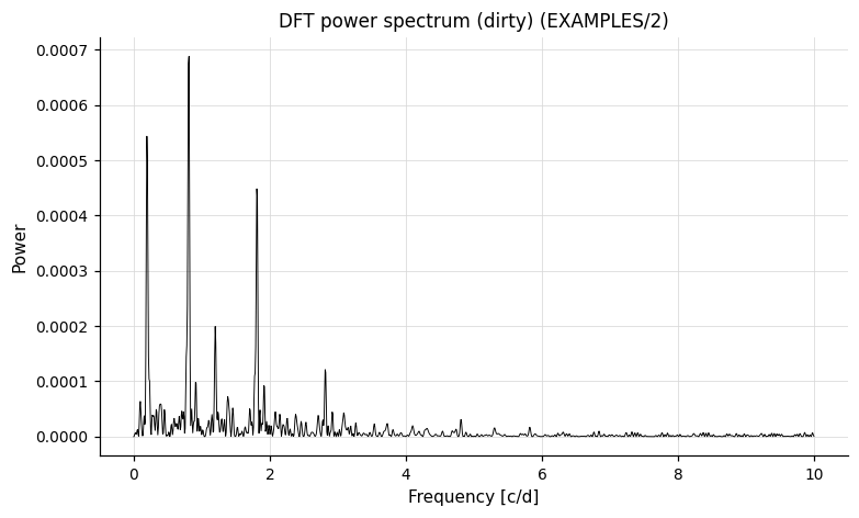
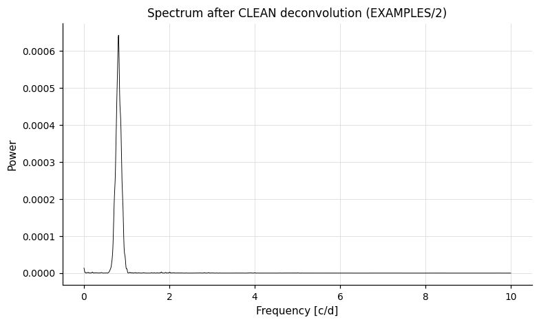
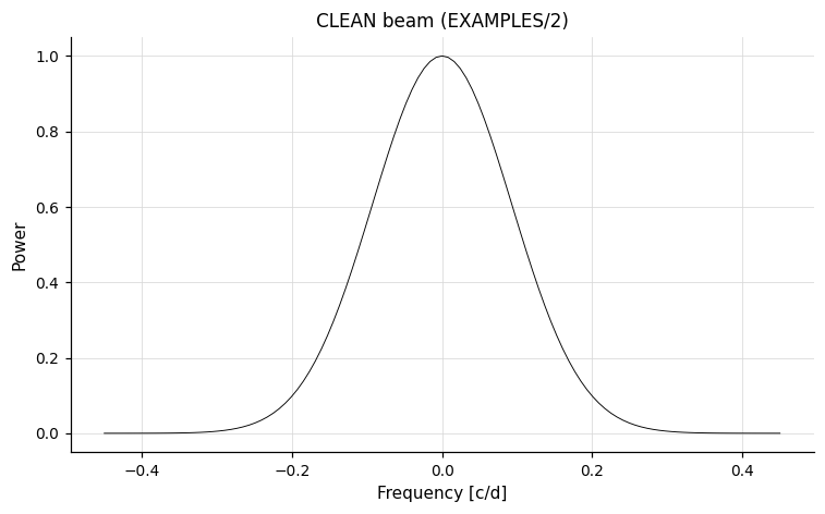
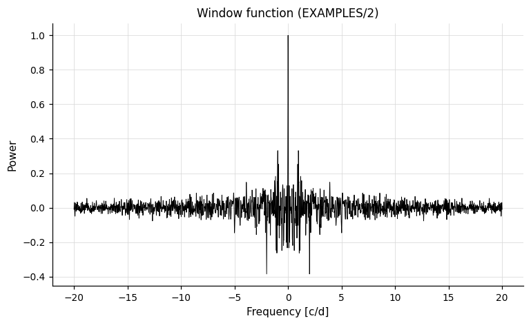
Example 2. Inject three harmonic signals into a light curve, compute the DFT, find the top 3 dirty-spectrum peaks, then apply the CLEAN algorithm and find the top 3 clean-spectrum peaks.

vartools -i EXAMPLES/4 -oneline -ascii \
    -Injectharm fix 0.697516 0 ampfix 0.1 phaserand 0 0 \
    -Injectharm fix 2.123456 0 ampfix 0.05 phaserand 0 0 \
    -Injectharm fix 0.426515 0 ampfix 0.01 phaserand 0 0 \
    -dftclean 4 maxfreq 10. outdspec EXAMPLES/OUTDIR1 \
        finddirtypeaks 3 clip 5. 1 \
        outwfunc EXAMPLES/OUTDIR1 \
        clean 0.5 5.0 outcbeam EXAMPLES/OUTDIR1 \
        outcspec EXAMPLES/OUTDIR1 \
        findcleanpeaks 3 clip 5. 1 \
        verboseout

The dirty spectrum, the spectrum after CLEAN deconvolution, the CLEAN beam, and the window function are written to EXAMPLES/OUTDIR1/:

---

-wwz — Weighted Wavelet Z-Transform

Syntax

-wwz <"maxfreq" <"auto" | "var" v | "expr" e | maxfreq>>
    <"freqsamp" <"var" v | "expr" e | freqsamp>>
    <"tau0" <"auto" | "var" v | "expr" e | tau0>>
    <"tau1" <"auto" | "var" v | "expr" e | tau1>>
    <"dtau" <"auto" | "var" v | "expr" e | dtau>>
    ["c" <"var" v | "expr" e | cval>]
    ["outfulltransform" outdir ["fits" | "pm3d"] ["format" format]]
    ["outmaxtransform" outdir ["format" format]]
    ["maskpoints" maskvar]

Description

Compute the Weighted Wavelet Z-Transform (WWZ) as defined by Foster (1996) using an abbreviated Morlet wavelet:

f(z) = exp(i·2π·f·(t-τ) - c·(2π·f)²·(t-τ)²)

The transform is computed for all combinations of trial frequency (up to maxfreq) and time shift (tau0 to tau1 in steps of dtau). This yields a time-frequency map of the signal power that is especially useful for non-stationary signals.

The decay constant c (default: 1/(8π²)) controls the trade-off between time and frequency resolution.

Python equivalent: wwz.

Parameters

Parameter	Description
"maxfreq" auto/val	Maximum frequency in cycles/day. "auto" = 1 / (2 · min_time_separation).
"freqsamp" freqsamp	Frequency sampling as a multiple of 1/T.
"tau0" auto/val	Start time for the time-shift scan. "auto" = minimum time in the light curve.
"tau1" auto/val	End time for the time-shift scan. "auto" = maximum time in the light curve.
"dtau" auto/val	Step size in time shift. "auto" = minimum time separation.
"c" cval	Morlet wavelet decay constant (default: 1/(8π²)).
"outfulltransform" outdir	Write the full 2D transform (time-shift × frequency) to outdir/$basename.wwz. Add "fits" for multi-extension FITS, or "pm3d" for gnuplot pm3d-compatible text format.
"outmaxtransform" outdir	Write the transform maximized over frequencies as a function of time-shift to outdir/$basename.mwwz.
"format" format	Override the default filename convention (same syntax as -o "nameformat").
"maskpoints" maskvar	Exclude points with maskvar ≤ 0.

Output columns

Column	Description
WWZ_maxZ_i	Maximum value of the Z-transform over all time-shifts and frequencies.
WWZ_maxfreq_i	Frequency corresponding to the maximum Z.
WWZ_maxpower_i	Power at the maximum Z.
WWZ_maxamp_i	Amplitude at the maximum Z.
WWZ_maxNeff_i	Effective number of data points at the maximum Z.
WWZ_maxtau_i	Time shift at the maximum Z.
WWZ_maxmeanmag_i	Local mean magnitude at the maximum Z.
WWZ_medZ_i	Median over time-shifts of the maximum-Z frequency's Z value.
(and corresponding med* columns for the other quantities)

References

Cite Foster 1996, AJ, 112, 1709.

Examples

Example 1. Compute the WWZ for EXAMPLES/8, scanning frequencies between 0 and 2.0 cycles per day at a step of 0.25/T (where T is the difference between the last and first observation times). Time-shifts run from the first observation to the last (tau0 and tau1 both auto) in steps of 0.1 days. The full 2-D transform is written to EXAMPLES/OUTDIR1/8.wwz in gnuplot pm3d format; the maximum-Z projection over frequency is written to EXAMPLES/OUTDIR1/8.mwwz. A significant periodic signal is seen near time 53735.17392 at a frequency of 0.30645 cyc/day, which is not present near the beginning or end of the time series.

vartools -i EXAMPLES/8 -oneline \
    -wwz maxfreq 2.0 freqsamp 0.25 tau0 auto tau1 auto dtau 0.1 \
        outfulltransform EXAMPLES/OUTDIR1/ pm3d \
        outmaxtransform EXAMPLES/OUTDIR1

A heat-map of the full transform can be generated in gnuplot with:

gnuplot> set pm3d map
gnuplot> unset key
gnuplot> splot "EXAMPLES/OUTDIR1/8.wwz" u 1:2:3

Or directly with matplotlib:

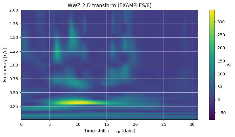
The transient ~0.3 cyc/day signal is clearly visible only between days 5–20 of the series.

---

-GetLSAmpThresh — Minimum Detectable Amplitude

Syntax

-GetLSAmpThresh
    < "ls" | "list" ["column" col] > minp thresh
    < "harm" Nharm Nsubharm | "file" listfile >
    ["noGLS"]

Description

Determine the minimum peak-to-peak amplitude that a signal at a given period must have to be detected by a Lomb-Scargle search with -ln(FAP) > thresh. The signal shape is either a Fourier series or read from a file. The threshold is computed by scaling the signal template until the LS statistic reaches the detection limit.

Python equivalent: GetLSAmpThresh.

Parameters

Parameter	Description
"ls"	Use the period from the most recent -LS command.
"list"	Read the period from the input list (optional "column" keyword).
minp	Minimum period that would be searched (sets the FAP scale).
thresh	Desired -ln(FAP) detection threshold.
"harm" Nharm Nsubharm	Describe the signal shape as a Fourier series with Nharm harmonics and Nsubharm sub-harmonics. The series is fit to the light curve at the specified period.
"file" listfile	Two-column file: signal_file signal_amp, one row per light curve. Each signal_file provides the signal magnitude in column 3; signal_amp is the peak-to-peak amplitude of that signal.
"noGLS"	Compute the threshold for the traditional (non-generalized) LS periodogram.

Output columns

Column	Description
GetLSAmpThresh_minfactor_i	Minimum factor by which the current signal must be scaled to remain detectable.
GetLSAmpThresh_minamp_i	Corresponding minimum peak-to-peak amplitude (magnitudes).

Examples

Example 1. Run LS to find the best period, extract the sinusoidal signal with -harmonicfilter, then compute the minimum detectable amplitude at that period given a threshold of -ln(FAP) > 100.

vartools -i EXAMPLES/2 -oneline \
    -LS 0.1 10. 0.1 1 0 \
    -harmonicfilter ls 0 0 0 fitonly \
    -GetLSAmpThresh ls 0.1 -100 harm 0 0

Output:

Name                                       = EXAMPLES/2
LS_Period_1_0                              =     1.23440877
Log10_LS_Prob_1_0                          = -4000.59209
LS_Periodogram_Value_1_0                   =    0.99619
LS_SNR_1_0                                 =   45.98308
HarmonicFilter_Mean_Mag_1                  =  10.12217
HarmonicFilter_Period_1_1                  =     1.23440877
HarmonicFilter_Per1_Fundamental_Sincoeff_1 =   0.05008
HarmonicFilter_Per1_Fundamental_Coscoeff_1 =  -0.00222
HarmonicFilter_Per1_Amplitude_1            =   0.10026
LS_AmplitudeScaleFactor_2                  =   0.02425
LS_MinimumAmplitude_2                      =   0.00243