Calling Python or R from VARTOOLS
VARTOOLS can invoke arbitrary user-supplied Python or R code on each
light curve (or on the full collection) via the -python and -R
commands. Both embed an interpreter at compile time, so the features are
only available if the corresponding development libraries were installed
when VARTOOLS was built (see the Installation page).
-R
Syntax
-R
    < "fromfile" commandfile | commandstring >
    ["init" < "file" initializationfile | initializationstring >
        | "continueprocess" prior_R_command_number]
    ["vars" variablelist
        | ["invars" inputvariablelist] ["outvars" outputvariablelist]]
    ["outputcolumns" variablelist] ["process_all_lcs"] ["verbose"]
Description
Execute arbitrary R code on each light curve. VARTOOLS embeds the user-supplied code in an R function and calls it once per light curve (or once for all light curves with "process_all_lcs"). Light-curve variables are passed to R as native R vectors.
Python equivalent: R.
Environment requirement
The R_HOME environment variable must be set before calling VARTOOLS. Find the correct value with R RHOME. Adding export R_HOME=$(R RHOME) to your .bashrc is recommended.
Parameters
| Parameter | Description |
|---|---|
"fromfile" commandfile |
Read R code from a file rather than the command line. |
commandstring |
R code as a single command-line string. |
"init" file initfile / "init" initstring |
R code executed once before processing (library imports, function definitions). |
"continueprocess" N |
Reuse the sub-process from the N-th prior -R (1-indexed). Shares state; no initialization code may be supplied. |
"vars" varlist |
Variables passed both into and received back from R. |
"invars" varlist |
Variables passed into R only. |
"outvars" varlist |
Variables received from R only. |
"outputcolumns" varlist |
Subset of out-vars to emit in the output statistics table. |
"process_all_lcs" |
Pass all light curves at once. Vectors arrive as lists of vectors; scalars as lists. |
"verbose" |
Allow R to print to stdout (default: R runs in --slave mode). |
Parallelism: under -parallel, a separate R sub-process is launched per thread; initialization runs independently for each thread, and globals are not shared between threads.
Examples
Example 1. Compute the standard deviation of the magnitudes of each light curve in EXAMPLES/lc_list using R. The expression b <- sd(mag) is evaluated for each LC; mag is passed in as a numeric vector and b is returned. The result is included as a column R_b_0 in the output table.
vartools -l EXAMPLES/lc_list -inputlcformat t:1,mag:2,err:3 -header \
    -R 'b <- sd(mag)' invars mag outvars b outputcolumns b
#Name R_b_0
EXAMPLES/1 0.15946976931434592
EXAMPLES/2 0.036640196913116818
EXAMPLES/3 0.0048962905656505422
EXAMPLES/4 0.0020915710522042882
EXAMPLES/5 0.002880850234933455
EXAMPLES/6 0.0020898736803245783
EXAMPLES/7 0.003488095003079855
EXAMPLES/8 0.0022502571019889705
EXAMPLES/9 0.0018673694762206033
EXAMPLES/10 0.0023627959129451301
Example 2. Same as Example 1 but using process_all_lcs to send the whole batch to R at once. Inside R the input vectors arrive as lists of vectors, and the output b must also be a list (with one entry per light curve).
vartools -l EXAMPLES/lc_list -inputlcformat t:1,mag:2,err:3 -header \
    -R 'b <- list(); for(i in 1:length(mag)) { b[[i]] <- sd(mag[[i]]); }' \
        invars mag outvars b outputcolumns b process_all_lcs
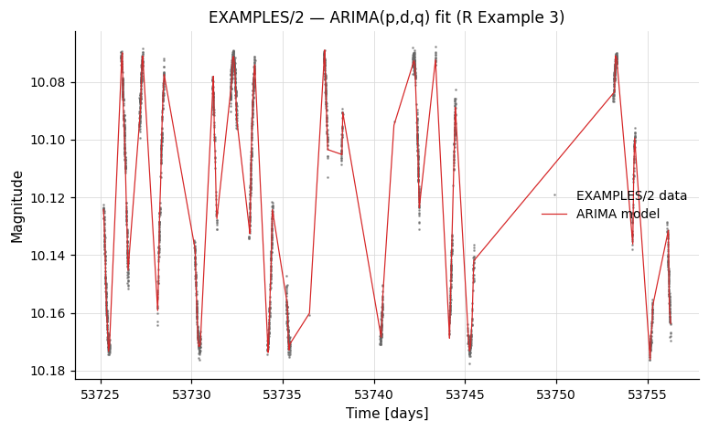
Example 3. ARIMA modelling of the light curves in EXAMPLES/lc_list using R's forecast package. (Note: ARIMA is being used here only to demonstrate the -R mechanics; it is not the recommended way to model these particular light curves.) After saving a copy of the input mag vector with -savelc, we bin and then resample the LC onto a uniform grid (ARIMA requires evenly-sampled data), call auto.arima to fit the model, subtract the residuals to obtain the smoothed model mag_arima, then resample back to the original time grid and restore the original mag. The output light curves include columns t, mag, mag_arima. Requires tseries and forecast to be installed in R.
vartools -l EXAMPLES/lc_list -inputlcformat t:1,mag:2,err:3 -header \
    -savelc \
    -binlc average binsize 0.05 taverage \
    -resample linear delt fix 0.05 \
    -R \
        'mag_ts <- ts(mag, start=1, end=length(t), frequency=1);
         arima_model <- auto.arima(mag_ts);
         mag_arima <- mag - as.vector(arima_model$residuals);' \
        init 'library(tseries); library(forecast);' \
        invars mag,t outvars mag_arima \
    -resample linear file list listcolumn 1 tcolumn 1 \
    -restorelc 1 vars mag \
    -o EXAMPLES/OUTDIR1 nameformat '%s.arimamodel' \
        columnformat t,mag,mag_arima
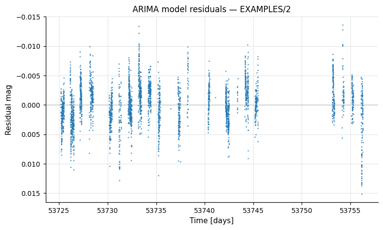
The output *.arimamodel files contain t, the original mag, and the smoothed mag_arima. Plotted against time, the model tracks the dominant variability in EXAMPLES/2; the residual mag − mag_arima is centred near zero:
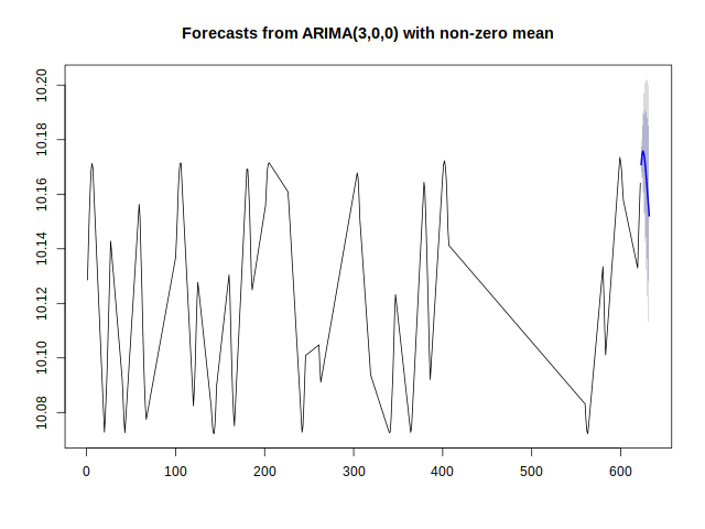
Example 4. Same as Example 3, but the ARIMA fit/forecast/residual diagnostics are wrapped in a function DoArimaFitPlot defined in EXAMPLES/Rexample4.R. We use -python to compute the LC basename (a stand-in for any place where Python's string handling is more convenient) and then call our R function with that basename. The function additionally writes *.arimaforecast.png and *.arimaresiduals.png plots to EXAMPLES/OUTDIR1. R diagnostic output is sent to stderr; append 2> /dev/null to silence it.
vartools -l EXAMPLES/lc_list -inputlcformat t:1,mag:2,err:3 -header \
    -savelc \
    -binlc average binsize 0.05 taverage \
    -resample linear delt fix 0.05 \
    -python 'lcbasename = Name.split("/")[-1]' \
        invars Name outvars lcbasename \
    -R 'mag_arima <- DoArimaFitPlot(mag, "EXAMPLES/OUTDIR1/", lcbasename)' \
        init file EXAMPLES/Rexample4.R \
        invars mag,t,lcbasename outvars mag_arima \
    -resample linear file list listcolumn 1 tcolumn 1 \
    -restorelc 1 vars mag \
    -o EXAMPLES/OUTDIR1 nameformat '%s.arimamodel' \
        columnformat t,mag,mag_arima
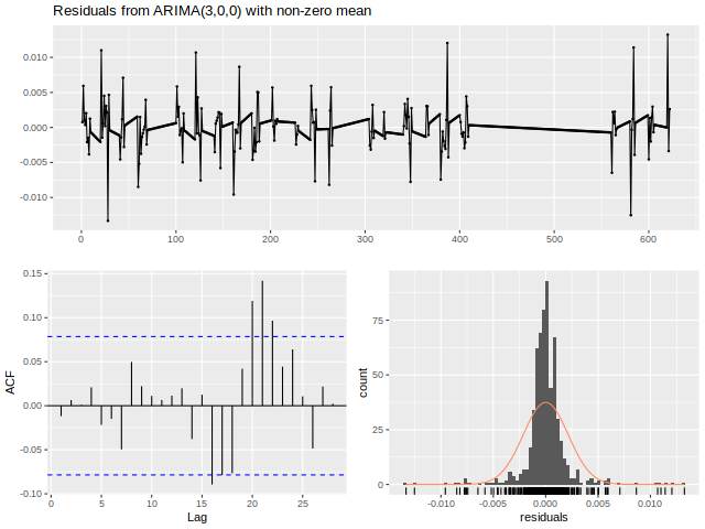
R's forecast::plot() and forecast::checkresiduals() calls inside DoArimaFitPlot produce the per-LC *.arimaforecast.png and *.arimaresiduals.png PNGs:
-python
Syntax
-python
    < "fromfile" commandfile | commandstring >
    ["init" < "file" initializationfile | initializationstring >
        | "continueprocess" prior_python_command_number]
    ["vars" variablelist
        | ["invars" inputvariablelist] ["outvars" outputvariablelist]]
    ["outputcolumns" variablelist] ["process_all_lcs"] ["skipfail"]
Description
Execute arbitrary Python code on each light curve. VARTOOLS embeds the user-supplied code in a Python function, compiles it via the Python C API, and calls it once per light curve. numpy is automatically imported. Numeric vectors arrive as numpy arrays; string data arrives as Python lists.
Parameters
| Parameter | Description |
|---|---|
"fromfile" commandfile |
Read Python code from a file rather than the command line. |
commandstring |
Python code as a single command-line string. |
"init" file initfile / "init" initstring |
Python code executed once before processing (function definitions, imports). |
"continueprocess" N |
Reuse the sub-process from the N-th prior -python (1-indexed). Shares state; no initialization may be supplied. |
"vars" varlist |
Variables passed both into and received back from Python. |
"invars" varlist |
Variables passed in only. |
"outvars" varlist |
Variables returned only. |
"outputcolumns" varlist |
Subset of out-vars to emit in the statistics table. |
"process_all_lcs" |
Pass all light curves at once. Numeric vectors arrive as lists of numpy arrays. |
"skipfail" |
On a per-LC exception, skip the remaining processing for that LC and continue. |
Parallelism: under -parallel, a separate Python sub-process is spawned per thread (sidestepping the GIL). Initialization runs independently for each thread.
Examples
Example 1. Compute the variance of each light curve's magnitudes in EXAMPLES/lc_list. The expression b = numpy.var(mag) is evaluated for each LC; mag arrives as a numpy array and b is returned. The result appears in the output table as PYTHON_b_0.
vartools -l EXAMPLES/lc_list -inputlcformat t:1,mag:2,err:3 -header \
    -python 'b = numpy.var(mag)' invars mag outvars b outputcolumns b
#Name PYTHON_b_0
EXAMPLES/1 0.025422461711037084
EXAMPLES/2 0.0013420988067623005
EXAMPLES/3 2.3966645306408949e-05
EXAMPLES/4 4.3733138204733634e-06
EXAMPLES/5 8.2971716866526236e-06
EXAMPLES/6 4.3664615059428104e-06
EXAMPLES/7 1.216345131566495e-05
EXAMPLES/8 5.0623773543353351e-06
EXAMPLES/9 3.4861868515750583e-06
EXAMPLES/10 5.5813996936871234e-06
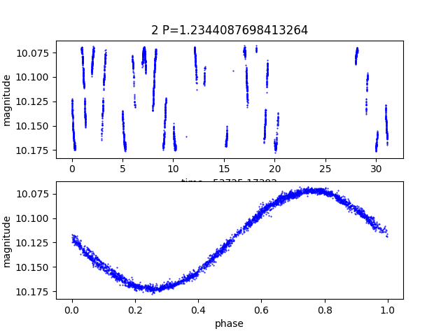
Example 2. Use matplotlib.pyplot to make a .png plot for each light curve with a sufficiently strong LS detection. The plotting function is defined in EXAMPLES/plotlc.py:
import matplotlib.pyplot as plt

def plotlc(lcname, outdir, t, ph, mag, P):
    lcbasename = lcname.split('/')[-1]
    plt.figure(1)
    plt.subplot(211)
    plt.gca().invert_yaxis()
    tcorr = t - t[0]
    plt.plot(tcorr, mag, 'bo', markersize=0.5)
    plt.ylabel('magnitude')
    plt.title(lcbasename + ' P=' + str(P))
    plt.xlabel('time - ' + str(t[0]))
    plt.subplot(212)
    plt.gca().invert_yaxis()
    plt.plot(ph, mag, 'bo', markersize=0.5)
    plt.ylabel('magnitude')
    plt.xlabel('phase')
    plt.savefig(outdir + '/' + lcbasename + '.png', format="png")
    plt.close()
vartools -l EXAMPLES/lc_list -inputlcformat t:1,mag:2,err:3 -header \
    -LS 0.1 100. 0.1 1 0 \
    -if 'Log10_LS_Prob_1_0<-100' \
        -Phase ls phasevar ph \
        -python 'plotlc(Name,"EXAMPLES/",t,ph,mag,LS_Period_1_0)' \
            init file EXAMPLES/plotlc.py \
    -fi
The init file keyword loads plotlc.py once; plotlc(...) is then called for each light curve that passes the -if condition. Running this on EXAMPLES/lc_list produces EXAMPLES/1.png and EXAMPLES/2.png. VARTOOLS must be compiled against a Python that can import matplotlib.
The plot below is the actual EXAMPLES/2.png produced by plotlc() — the LC vs time on the top panel, phase-folded at the LS period on the bottom:
Example 3. Same as Example 2, but use process_all_lcs to plot every light curve in a single Python call. With process_all_lcs enabled, vector inputs (t, ph, mag) arrive as lists of numpy arrays, scalar inputs (Name, LS_Period_1_0) arrive as numpy arrays, so the loop steps through each light curve manually.