The VARTOOLS program is a command line utility that provides tools for processing and analyzing astronomical time series data, especially light curves. It includes methods for calculating variability/periodicity statistics of light curves; for filtering, transforming, and otherwise modifying light curves; and for modeling light curves. It is intended primarily for batch processing a large number of light curves. The program is run by issuing a sequence of commands to perform actions on light curves, each command is executed in turn with the resulting light curves passed to the next command. Statistics computed by each command are sent to stdout as an ascii table.
This program is available without any warranty - use it at your own risk. If you do find a bug, please let me know so that I can fix it (jhartman AT astro DOT princeton DOT edu). Also feel free to let me know if there are any commands/algorithms that you would like to see added to this program.
Citation: If you use this program, please cite Hartman and Bakos, 2016, Astronomy and Computing, 17, 1, which provides the scientific and technical reference for this program. Also, be sure to cite the relevant sources for the algorithms that you use. The paper describes version 1.33.
You can add your own commands to VARTOOLS by developing them as libraries that can be dynamically linked at runtime. See the ReadME file in the USERLIBS subdirectory for details. If you have any troubles getting it to work, or if its not clear how to write the wrapper for the processing algorithm you are trying to include, please let me know. Also, if you develop your own command and would like to share it with people, I would be happy to include it in the distribution if it works. You can also use the -python and -R commands to execute PYTHON or R routines on light curves through VARTOOLS.Download Version 1.51 (Released May 27, 2025)
The development version of VARTOOLS can also be obtained from the VARTOOLS github repository
Follow the installation instructions. VARTOOLS uses the GNU auto-build system for configuration and compilation. Version 1.38 has been successfully built on Linux and Mac systems, and should also work on Windows machines using MinGW. Note that the -python command and -R commands have only been tested under Linux and Mac and may not work on windows. See step-by-step instructions for installing VARTOOLS on macOS Mojave 10.14.3. See also notes on installing an older version on a Windows machines using MinGW, thanks to Arthur Sweeney at the University of Dallas. The Mac and Windows notes may be useful for instructions on how to install libraries and the build tools needed.
Development of VARTOOLS was supported by NASA grant NNX14AE87G
Commands: In the current version, the following commands are supported:
-addfitskeyword
    keyword
    ["combinelc" lcnumvar]
    < "TDOUBLE" | "TINT" | "TLONG" | "TSTRING" >
    < "fix" val | "var" variable >
    ["comment" commentstring]
    ["primary" | "extension"]
    ["append" | "update"]
Add a keyword to the header of any subsequently output fits-format light curves. Parameters are as follows:
keyword - The header keyword to add.
"combinelc" lcnumvar - optionally add multiple keywords, one per value of the lcnumvar variable. In this case 'keyword' should be a format rule with instances of "%d" replaced with the unique values of lcnumvar. If using the "var" option below, the value of that variable will be evaluated at the first instance in the light curve where lcnumvar takes on a new unique value. Use this option for example, to log the values of a combinelc variable specified with "-inlistvars" into a light curve header.
"TDOUBLE" | "TINT" | "TLONG" | "TSTRING" - The datatype to use for the keyword
"fix" val - set the value to a fixed value set on the command-line for all light curves.
"var" variable - set the value to the contents of a variable.
"comment" commentstring - optionally include a comment string for this header keyword.
"primary" | "extension" - by default the keyword will be appended to the end of the primary header. Optionally put it at the end of the header for the table extension by using the "extension" option, or explicitly set it to the primary header by using the "primary" option.
"append" | "update" - by default, if the keyword already exists in the header, it will be updated. Optionally append the same keyword again if it already exists by using the "append" option, or set the "update" option to explicitly indicate this behavior.
-addnoise
    <   "white"
                <"sig_white" <"fix" val | "list" ["column" col]>>
      | "squareexp"
                <"rho" <"fix" val | "list" ["column" col]>>
                <"sig_red" <"fix" val | "list" ["column" col]>>
                <"sig_white" <"fix" val | "list" ["column" col]>>
                ["bintime" <"fix" val | "list" ["column" col]>]
      | "exp"
                <"rho" <"fix" val | "list" ["column" col]>>
                <"sig_red" <"fix" val | "list" ["column" col]>>
                <"sig_white" <"fix" val | "list" ["column" col]>>
                ["bintime" <"fix" val | "list" ["column" col]>]
      | "matern"
                <"nu" <"fix" val | "list" ["column" col]>>
                <"rho" <"fix" val | "list" ["column" col]>>
                <"sig_red" <"fix" val | "list" ["column" col]>>
                <"sig_white" <"fix" val | "list" ["column" col]>>
                ["bintime" <"fix" val | "list" ["column" col]>]
      | "wavelet"
                <"gamma" <"fix" val | "list" ["column" col]>>
                <"sig_red" <"fix" val | "list" ["column" col]>>
                <"sig_white" <"fix" val | "list" ["column" col]>>
    >
Add time-correlated noise to the light-curve. The noise is assumed to be Gaussian. The user must specify the model to be assumed for time correlations. Options include:
"white" - pure white noise without a time-correlated component. This noise is parameterized by the standard deviation, sig_white.
"squareexp" - a Gaussian-process with a squared-exponential covariance matrix. The covariance between times t_i and t_j is given by sig_white^2*delta_ij + sig_red^2*exp(-(t_i-t_j)^2/2/rho^2) where delta_ij is the Kronecker delta function, and sig_white, sig_red and rho are parameters of the model. Note that rho and sig_red must both be greater than zero. The sig_white term allows for an additional noise component that is uncorrelated in time. The optional "bintime" keyword can be used to chunk the light curve into time bins of a specified duration and independently simulate the correlated noise in each bin. This can speed up the simulations substantially in cases where the full light curve duration is much longer than the correlation timescale.
"exp" - a Gaussian-process with an exponentially decaying covariance matrix. The covariance between times t_i and t_j is given by sig_white^2*delta_ij + sig_red^2*exp(-(t_i-t_j)/rho) where delta_ij is the Kronecker delta function, and sig_white, sig_red and rho are parameters of the model. Note that rho and sig_red must both be greater than zero. The sig_white term allows for an additional noise component that is uncorrelated in time. The optional "bintime" keyword can be used to chunk the light curve into time bins of a specified duration and independently simulate the correlated noise in each bin. This can speed up the simulations substantially in cases where the full light curve duration is much longer than the correlation timescale.
"matern" - a Gaussian-process with a Matern covariance matrix. The covariance between times t_i and t_j is given by sig_white^2*delta_ij + sig_red^2*C(nu,x)*K_nu(x) with x=sqrt(2*nu)*(|t_i-t_j|)/rho and C(x,y)=(2^(1-x)/Gamma(x))*(y)^x with K_nu being the modified Bessel function of the second kind, and Gamma the usual gamma function. In this case the parameters are nu, rho, sig_white, and sig_red. All but sig_white must be greater than zero. The sig_white term allows for an additional noise component that is uncorrelated in time. The optional "bintime" keyword can be used to chunk the light curve into time bins of a specified duration and independently simulate the correlated noise in each bin. This can speed up the simulations substantially in cases where the full light curve duration is much longer than the correlation timescale.
"wavelet" - the sum of a red-noise component with power-spectral-density proportional to 1/f^gamma (gamma must satisfy -1 < γ < 1) with standard deviation σ_red, and a white noise component with standard deviation σ_white. The red-noise is generated using the method of McCoy and Walden, 1996, Journal of Computational and Graphical Statistics, Vol 5, No. 1, pp. 26-56 (section 4.2).
For each of the parameters one may either use the "fix" keyword and specify the value on the command-line, or use the "list" keyword in which case the value is read-in from the input list (optionally give the column in the list with the "column" keyword, if not specified the next free column is assumed).
-alarm
    ["maskpoints" maskvar]
Calculate the alarm variability statistic for each light curve. Optionally use the "maskpoints" keyword and provide the name of a vector to mask out points in the light curve from the calculation. Points in each light curve with maskvar > 0 will be included in the calculation, while others will be excluded. Cite Tamuz, Mazeh, and North 2006, MNRAS, 367, 1521 if you use this tool. Cite Tamuz, Mazeh, and North 2006, MNRAS, 367, 1521 if you use this tool.
-aov
    ["Nbin" <"var" Nbinvar | "expr" Nbinexpr | Nbin>]
    <"var" minpvar | "expr" minpexpr | minp>
    <"var" maxpvar | "expr" maxpexpr | maxp>
    <"var" subsamplevar | "expr" subsampleexpr | subsample>
    <"var" finetunevar | "expr" finetuneexpr | finetune>
    Npeaks operiodogram [outdir]
    ["whiten"] ["clip" clip clipiter] ["uselog"]
    ["fixperiodSNR" <"aov" | "ls" | "injectharm" | "fix" period
        | "list" ["column" col]
        | "fixcolumn" <colname | colnum>>]
    ["maskpoints" maskvar]
Perform an Analysis of Variance (AoV) period search on the light curves using phase binning. Specify "Nbin" and a number to change the number of bins used from the default value of 8. minp and maxp are the minimum and maximum periods to search. The initial search will use a frequency resolution of subsample/T where T is the baseline of the light curve. The peak periods will be refined using a resolution of finetune/T. For Nbin, minp, maxp, subsample and finetune, optionally use the "var" or "expr" keyword to set the parameter to the value of a variable or an analytic expression, otherwise just give the value on the command-line to fix it for all light curves. The program will output the Npeaks highest peaks in the periodogram of the light curve. By default the program will output, for each peak, the period, the θ_aov statistic, the signal to noise ratio (θ_aov - <θ_aov>)/RMS(θ_aov), and -ln(FAP) where FAP is the formal false alarm probability (this is calculated from the value of θ_aov using the Horne and Baliunas 1986, ApJ, 302, 757 estimate for the bandwidth penalty).
operiodogram should be either 0 or 1. If it is set to 1 then the periodogram for each light curve will also be output to the directory outdir, with the suffix ".aov". The first column in the output is the period, the second column is θ_aov.
If the "whiten" keyword is given, then the light curve will be whitened at each peak period and the periodogram will be recomputed before searching for the next peak period. The values of <θ_aov> and RMS(θ_aov) used for each peak are computed on the whitened periodogram. The output spectrum will contain the Npeaks separate periodograms.
Use the "clip" keyword to change the clipping parameters for calculating the average and RMS of the power spectrum when computing the SNR value of a peak. clip is the sigma-clipping factor, and clipiter is a flag that is 1 or 0 to toggle iterative clipping. By default iterative 5-sigma clipping is used.
Use the keyword "uselog" to output the ln(θ_aov) SNR instead of the standard statistics (this is the original behavior for this command), i.e. the statistic is (<-ln(θ_aov)> - ln(θ_aov))/RMS(-ln(θ_aov)) where the average and RMS are taken over the entire periodogram for a light curve. In this case the output will also include the average and RMS of -ln(θ_aov).
Use the "fixperiodSNR" option to output the AoV statistic, SNR etc at a specified period. See the help for the "-LS" command for an explanation of the syntax.
Optionally use the "maskpoints" keyword and provide the name of a vector to mask out points in the light curve from the calculation of the periodogram. Points in each light curve with maskvar > 0 will be included in the calculation, while others will be excluded.
Cite Schwarzenberg-Czerny, A., 1989, MNRAS, 241, 153 and Devor, J., 2005, ApJ, 628, 411 if you use this tool. (The Devor citation is needed because this code is based on his implementation of AoV).
-aov_harm
    <"var" Nharmvar | "expr" Nharmexpr | Nharm>
    <"var" minpvar | "expr" minpexpr | minp>
    <"var" maxpvar | "expr" maxpexpr | maxp>
    <"var" subsamplevar | "expr" subsampleexpr | subsample>
    <"var" finetunevar | "expr" finetuneexpr | finetune>
    Npeaks operiodogram [outdir]
    ["whiten"] ["clip" clip clipiter]
    ["fixperiodSNR" <"aov" | "ls" | "injectharm" | "fix" period
        | "list" ["column" col]
        | "fixcolumn" <colname | colnum>>]
    ["maskpoints" maskvar]
Perform an Analysis of Variance (AoV) period search on the light curves using a multi-harmonic model. The parameters and behavior are as for the "-aov" command. In this case the model signal is a harmonic function with Nharm harmonics. If Nharm is < 1 then it will be automatically varied until the false alarm probability, which includes a penalty for overfitting the data, is minimized.
Cite Schwarzenberg-Czerny, A., 1996, ApJ, 460, L107 if you use this tool.
-autocorrelation
    start stop step outdir ["maskpoints" maskvar]
Calculate the discrete auto-correlation function (Edelson and Krolik 1988, ApJ, 333, 646), these are written out to outdir"/"$basename".autocorr", where $basename is the base filename of the input light curve.
start, stop and step are the times in days for sampling the auto-correlation. Note that rather than using the variance of the light curve in the denominator, we use the formal uncertainty (we do not subtract the "measurement error" from the variance as done in the Edelson and Krolik formula since this could lead to imaginary numbers in the case where measurement errors are overestimated). If you wish to use the variance in the denominator rather than the formal uncertainty you should issue the "-changeerror" command before calling this routine. Note that due to binning, when the variance used in the denominator the autocorrelation function may be smaller than 1 unless the time step used is less than the time difference between any consecutive measurements in the light curve.
Optionally use the "maskpoints" keyword and provide the name of a vector to mask out points in the light curve from the calculation. Points in each light curve with maskvar > 0 will be included in the calculation, while others will be excluded.
-binlc
    <"average" | "median" | "weightedaverage">
    <"binsize" binsize | "nbins" nbins>
    ["bincolumns" var1[:stats1][,var2[:stats2],...]]
    ["T0"
        <"fix" T0val | "list" ["column" col] | "fixcolumn" <colname | colnum> |
         "expr" expression>]
    ["firstbinshift" firstbinshift]
    <"tcenter" | "taverage" | "tmedian" | "tnoshrink" ["bincolumnsonly">
    ["maskpoints" maskvar]
Bin the light curves in time (or phase if a "-Phase" command has already been issued). Use the average keyword to take the average of points in a bin, median to take the median of the points, or weightedaverage to take the weighted average (for backward compatibility, you can also use the numbers 0, 1 or 2). One should specify either the binsize in units of the time coordinate (e.g. in phase if the light curves have been phased), or nbins, which is the number of bins to split the light curve time-span into. By default all other columns in the light curve will be binned in the same way, you can optionally change the binning type for some of the columns using the bincolumns keyword. If you do this, then the string of the form var1[:stats][,var2[:stats2],...] is a comma separated list of variable names, with a statistics name appended to each variable following a ":". The choices for statistics are the same as for the "-stats" command. By default the first bin begins at the initial time in the light curve (t0), if firstbinshift is specified, then this will be shifted by t0 - firstbinshift/binsize. Alternatively, if the "T0" keyword is used, then the user may specify the start of the first time bin for each light curve. The options here are "fix" to fix the parameter to a value given on the command-line, "list" to have the parameter read-in from the input light curve list (optionally giving the column number with the keyword "column", by default the next column in the list is used), "fixcolumn" to use a previously computed column from the output statistics file, or "expr" to set the value to an analytic expression which is evaluated for each light curve at the time this command is executed. Note that if the specified T0 is greater than the latest time in the light curve, the number of points in the resulting light curve is set to zero. If T0 is greater than the initial time in the light curve, but smaller than the final time in the light curve, then any observations with time less than T0 will be added to the first bin. If the tcenter keyword is given then the output time for each bin is the time at the center of the bin, if taverage is given then the time will be the average of the times of points that fall within the bin, if tmedian is given then the time will be the median of the times of points in the bin, and if tnoshrink is given then the size of the light curve will not be reduced by the binning, and instead all points in the light curve will be replaced by the binned value (for backward compatability, you can also use the numbers 0, 1, 2, or 3). If you only want to apply the binning to some of the columns in the light curve, but not all of them, you can give the tnoshrink keyword followed by bincolumnsonly. In this case only the variables explicitely listed after bincolumns will be binned (this includes t, mag and err).
Optionally use the "maskpoints" keyword and provide the name of a vector to use in masking out points in the light curve from the calculation. Points with maskvar > 0 will be included in the binning, while others will be excluded. Note that if tnoshrink is given, then the binned values will still be calculated and reported at the masked-out times, but the masked points will not contribute themselves to the calculated binned values.
-BLS
    < "r" <"var" rminvar | "expr" rminexpr | rmin>
             <"var" rmaxvar | "expr" rmaxexpr | rmax> |
      "q" <"var" qminvar | "expr" qminexpr | qmin>
          <"var" qmaxvar | "expr" qmaxexpr | qmax> |
      "density" <"var" rhovar | "expr" rhoexpr | rho>
                <"var" minexpdurfracvar | "expr" minexpdurfracexpr | minexpdurfrac>
                <"var" maxexpdurfracvar | "expr" maxexpdurfracexpr | maxexpdurfract> >
    < "var" minpervar | "expr" minperexpr | minper >
    < "var" maxpervar | "expr" maxperexpr | maxper >
    < "nf" <"var" nfreqvar | "expr" nfreqexpr | nfreq> |
      "df" <"var" dfreqvar | "expr" dfreqexpr | dfreq> |
      "optimal" <"var" subsamplevar | "expr" subsampleexpr | subsample>>
    < "var" nbinsvar | "expr" nbinsexpr | nbins>
    timezone Npeak outperiodogram [outdir] omodel [modeloutdir]
    correctlc ["extraparams"] ["fittrap"] ["nobinnedrms"]
    ["ophcurve" outdir phmin phmax phstep]
    ["ojdcurve" outdir jdstep]
    ["stepP" | "steplogP"]
    ["adjust-qmin-by-mindt" ["reduce-nbins"]]
    ["reportharmonics"] ["maskpoints" maskvar]
This command runs the Box-Least Squares (BLS) transit search algorithm on the light curves. You may either set a fixed minimum and maximum q (fraction of orbit in transit) for the search, you can specify a minimum and maximum stellar radius r to consider (in solar radii) in which case the qmin and qmax values are calculated from the input rmin and rmax values, for each trial period P, using q = 0.076 * R^(2/3) * P^(-2/3) (with P in days; this assumes R = M as an approximation for the lower main sequence), or you can specify a stellar density (in grams per cubic centimeter) and a minimum and maximum fraction of the expected transit duration (assuming a circular orbit) to consider. For all of these parameters either give the value on the command-line that will be used for processing all light curves, give the "var" keyword followed by the name of a previously created variable that will hold the value to use for each light curve, or give the "expr" keyword to evaluate an analytical expression to determine the value to use for each light curve.
The minimum and maximum periods to search (minper and maxper) are given in days (again either give the values on the command line, or use the "var" or "expr" keywords to give a variable or expression to evaluate to determine the values).
Give either the "nf" keyword, the "df" keyword, or the "optimal" keyword to specify the number of trial frequencies, the frequency step-size, or to use Ofir's optimal frequency spacing. For the optimal method the density option must be used, and the subsampling factor should be specified. Use the "var" or "expr" keywords to provide a variable or analytic expression that returns the value to use, or just give the parameter value on the command-line if fixing it for all light curves. The appropriate number to use for nfreq depends on the minimum transit duration you are considering, and the timespan of the observations. If T is the timespan of the observations, qmin is the minimum fractional transit duration to consider, then a rough estimate for df = (f_max - f_min)/Nfreq is df = 0.25qmin/T.
nbins is the number of phase bins to break the light curve into (this should be at least 2/qmin). Either give the value on the command-line, or use the "var" or "expr" keywords to provide a variable or expression.
timezone is the number (in hours) to add to add to UTC to get the local time (-7 for Arizona). This is used to determine which nights different observations come from and thus to determine the fraction of Δχ² that comes from a single night. If observations come from multiple sites, set this to 0 and ignore the output for the fraction of Δχ² from one night.
Npeak is the number of peaks in the BLS spectrum to find and report.
outperiodogram is a flag that is set to 1 to output the BLS period vs. SN spectrum.
outdir is the output directory for the BLS spectrum if outperiodogram is set to 1, ".bls" will be appended to the filename.
omodel is a flag set to 1 or zero that can be used to output the model for the light curve, the output directory is then given in modeloutdir, the suffix ".bls.model" will be appended to the filename.
correctlc is either 0 or 1, set to 1 it will subtract the transit model from the light curve before passing it to the next command.
If the optional "extraparams" keyword is given, then a number of additional parameters that could be useful for culling false positives will be included in the output table.
If the optional "fittrap" keyword is specified, the routine will fit a trapezoidal transit to each BLS peak. This allows a refined estimate of the transit time, duration and depth. In this case the output table will also include qingress which is the fraction of the transit duration covered by ingress, a value of 0 corresponds to a perfectly box-shaped transit, a value of 0.5 corresponds to a V-shaped transit.
The optional keyword "nobinnedrms" adjusts the way in which the BLS_SN statistic is calculated. When "nobinnedrms" is given the procedure runs faster, but the SN will tend to be suppressed for high significance detections. If this option is given use another parameter (Δχ² or signal-to-pink-noise) for selecting transits rather than BLS_SN. Note that in some cases the default behavior will supress the signal at very high peaks (characterized by the periodogram going to zero in the center of a peak), to avoid this behavior use the "nobinnedrms" keyword.
If the optional keyword "ophcurve" is given then a model phase curve will be output to a file in the directory outdir with suffix ".bls.phcurve". It will be generated with phases between phmin and phmax and a uniform step size of phstep.
If the optional keyword "ojdcurve" is given then a model light curve will be output to a file in the directory outdir with suffix ".bls.jdcurve". The times will be between the first and last times in the light curve with a uniform step size of jdstep.
By default the BLS spectrum is sampled at uniform frequency steps. To sample it at uniform steps in period or log(period) use the "stepP" or "steplogP" keyword.
Use the optional "adjust-qmin-by-mindt" keyword to adaptively set the minimum q value to the maximum of qmin or mindt*frequency where mindt is the minimum time difference between consecutive points in the light curve. If this keyword is given you may also use the "reduce-nbins" keyword to adaptively reduce the number of phase bins at each frequency such that there are no more than 2 bins to sample a transit of duration qmin. By default any peak in the spectrum at a frequency that is a lower order rational multiple of a frequency with a higher peak will not be reported. To report these harmonic frequencies use the "reportharmonics" keyword.
Optionally use the "maskpoints" keyword and provide the name of a vector to mask out points in the light curve from the calculation of the BLS spectrum. Points in each light curve with maskvar > 0 will be included in the calculation, while others will be excluded. If correctlc=1, then the BLS model will be subtracted from all points in the light curve, including those with maskvar <= 0. If omodel=1, the output model file will only include the model evaluated at points with maskvar > 0.
Cite Kovács, G., Zucker, S., & Mazeh, T. 2002, A&A, 391, 369 if you use this tool. The reference for the optimal frequency sampling is Ofir, A. 2014, A&A, 561, A138.
-BLSFixDurTc
    <"duration" <"fix" | "fixcolumn" <colname | colnum>
        | "list" ["column" col]>>
    <"Tc" <"fix" | "fixcolumn" <colname | colnum>
        | "list" ["column" col]>>
    ["fixdepth" <"fix" depth | "fixcolumn" <colname | colnum>
        | "list" ["column" col]>
        ["qgress" <"fix" qgress | "fixcolumn" <colname | colnum>
            | "list" ["column" col]>]]
    minper maxper nfreq timezone
    Npeak outperiodogram [outdir] omodel [model_outdir]
    correctlc ["fittrap"]
    ["ophcurve" outdir phmin phmax phstep]
    ["ojdcurve" outdir jdstep]
    ["maskpoints" maskvar]
This command runs BLS on a light curve fixing the duration of the transit and a reference time of transit (use the "duration" and "Tc" keywords, respectively). Optionally the depth and ingress duration may be fixed as well ("fixdepth" and "qgress" parameters. Note that for the ingress duration, what is specified is the fraction of transit that is covered by ingress. For a grazing transit this is 0.5). For each of these parameters the value to use can be fixed to the value given on the command-line, it can be set to a value calculated from a previously executed command and reported in the output ascii table ("fixcolumn" followed by either the heading name or column number) or it can be read-in from the input "list" file. The remaining options are as for the "-BLS" command.
Cite Kovács, G., Zucker, S., & Mazeh, T. 2002, A&A, 391, 369 if you use this tool.
-BLSFixPer
    <"aov" | "ls" | "list" ["column" col]
        | "fix" period | "fixcolumn" <colname | colnum>
        | "expr" expr>
    <"r" rmin rmax | "q" qmin qmax >
    nbins timezone omodel [model_outdir] correctlc ["fittrap"]
    ["maskpoints" maskvar]
This command runs BLS at a fixed period on the light curves - it searches merely for the most transit-like signal at the specified period. The period comes either from the last aov command, from the last ls command, is specified in the input-list (keyword list; by default it will be taken from the next available column, use the "column" keyword to specify the column), is fixed to the value given on the command-line for all light curves, is set to the value output by a previously executed command (using "fixcolumn"), or is set to the value of an analytic expression.
Like BLS you can either specify a minimum and maximum stellar radius r to consider, or a minimum and maximum q to consider. Similarly you must specify the number of bins to use (nbins)and the timezone.
omodel is 1 to output the model light curve to model_outdir (with ".blsfixper.model" appended to the end of the file name.
correctlc is 1 to subtract the transit model from the light curve before passing it to the next command.
"fittrap" is an optional keyword, which if specified, fits a trapezoidal transit after running the BLS scan.
Optionally use the "maskpoints" keyword and provide the name of a vector to mask out points in the light curve from the calculation of the BLS statistic. Points in each light curve with maskvar > 0 will be included in the calculation, while others will be excluded. If correctlc=1, then the BLS model will be subtracted from all points in the light curve, including those with maskvar <= 0. If omodel=1, the output model file will only include the model evaluated at points with maskvar > 0.
Cite Kovács, G., Zucker, S., & Mazeh, T. 2002, A&A, 391, 369 if you use this tool.
-BLSFixPerDurTc
    <"period" <"fix" per | "fixcolumn" <colname | colnum>
        | "list" ["column" col]>>
    <"duration" <"fix" dur | "fixcolumn" <colname | colnum>
        | "list" ["column" col]>>
    <"Tc" <"fix" Tc | "fixcolumn" <colname | colnum>
        | "list" ["column" col]>>
    ["fixdepth" <"fix" depth | "fixcolumn" <colname | colnum>
        | "list" ["column" col]>
        ["qgress" <"fix" qgress | "fixcolumn" <colname | colnum>
            | "list" [column" col]>]]
    timezone omodel [model_outdir]
    correctlc ["fittrap"]
    ["ophcurve" outdir phmin phmax phstep]
    ["ojdcurve" outdir jdstep] ["maskpoints" maskvar]
This command runs BLS at a fixed period, transit duration and epoch on the light curves. Options are similar to -BLSFixDurTc, except that the period must also be specified.
Cite Kovács, G., Zucker, S., & Mazeh, T. 2002, A&A, 391, 369 if you use this tool.
-changeerror
    ["maskpoints" maskvar]
Replace the formal errors in a light curve with the RMS of the light curve.
Optionally use the "maskpoints" keyword and provide the name of a vector to mask out points in the light curve from the RMS calculation. Points with maskvar > 0 will be included in the calculation, while others will be excluded.
-changevariable
    <"t" | "mag" | "err" | "id"> var
Change the variable used for time, magnitude, magnitude uncertainty, or image-id (keywords: "t", "mag", "err" and "id", respectively) in subsequent commands. First specify what is being changed, and then give the name of the variable which will now fulfill this role.
Suppose for example that you have read in the variables mag and mag2 using the -inputlcformat option. After "-changevariable mag mag2" is issued, subsequent commands will use mag2 for the magnitudes rather than mag. The variable mag will still exist, if you wish to switch back to using mag for the magnitudes, you should issue the command "-changevariable mag mag".
-chi2
    ["maskpoints" maskvar]
Calculate χ² per degree of freedom for the light curves. The output will include χ²/dof and the error weighted mean magnitude.
Optionally use the "maskpoints" keyword and provide the name of a vector to mask out points in the light curve from the calculation. Points with maskvar > 0 will be included in the calculation, while others will be excluded.
-chi2bin
    Nbin bintime1...bintimeNbin
    ["maskpoints" maskvar]
Calculate χ²/dof after applying a moving mean filter to the light curves. Note that the light curves passed to the next command are unchanged. Nbin filters are used (with Nbin resulting estimates of χ²/dof and the error weighted mean). The width of filter 1 is given by 2.0*bintime1, and similarly for other filters (the bintimes are given in minutes).
Optionally use the "maskpoints" keyword and provide the name of a vector to mask out points in the light curve from the calculation. Points with maskvar > 0 will be included in the calculation, while others will be excluded.
-clip
    sigclip iter ["niter" n] ["median"]
    ["markclip" var ["noinitmark"]]
Sigma-clip the light curves using a clipping factor of sigclip. iter is a flag that is either 1 for iterative clipping (performed continuously until no further points are removed), or 0 to not do continuous iterative clipping. To clip for a fixed number of iterations give the "niter" keyword followed by the number of iterations to use. By default clipping is done with respect to the mean. To use the median instead provide the "median" keyword. The output table will include the number of points that were clipped. Note that points with errors <= 0 or with NaN magnitude values will be clipped. If sigclip is <= 0, then sigma-clipping is not performed, but points with errors <= 0 or with NaN magnitude values will be clipped.
By default clipped points will be removed from the light curve. If the "markclip" keyword is given, then the points will not be removed, but instead points that would not be clipped will have var set to 1, while points that would be clipped will have var set to 0. By default the program will ignore any prior values that may be set in the var variable. If the "noinitmark" keyword is given after the variable name, then the input var values will be taken as an initial clipping mask, and only points with var = 1 will be considered in calculating additional points to clip.
-converttime
    <"input" <"mjd" | "jd" | "hjd" | "bjd" >>
    ["inputsubtract" value] ["inputsys-tdb" | "inputsys-utc"]
    <"output" <"mjd" | "jd" | "hjd" | "bjd" >>
    ["outputsubtract" value] ["outputsys-tdb" | "outputsys-utc"]
    ["radec" <"list" ["column" col] | "fix" raval decval |
            "expr" raexpr decexpr | "perJD expr" raexpr decexpr |
            "perJD fromlc" ralccol declccol>
        ["epoch" epoch]]
    ["ppm" <"list" ["column" col] | "fix" mu_ra mu_dec>]
    ["input-radec" <"list" ["column" col] | "fix" raval decval |
            "expr" raexpr decexpr | "perJD expr" raexpr decexpr |
            "perJD fromlc" ralccol declccol>
        ["epoch" epoch]]
    ["input-ppm" <"list" ["column" col] | "fix" mu_ra mu_dec>]
    ["ephemfile" file] ["leapsecfile" file] ["planetdatafile" file]
    ["observatory" < code | "show-codes">
        | "coords" ["xyz"]
            <"fix" latitude[deg] longitude[deg_E] altitude[m]
            | "list" ["column" collat collong colalt]
            | "expr" [latexpr longexpr altexpr]
            | "fromlc" collat collong colalt
            | "lcexpr" [latexpr longexpr altexpr]>]
Convert the time system of the light curves. The user must specify "input" followed by the input time system (options are "mjd" = modified Julian date, "jd" = Julian date, "hjd" = Helio-centric Julian date, or "bjd" = Bary-centric Julian date). The "bjd" option is only available if VARTOOLS has been linked to the JPL NAIF cspice library (available from http://naif.jpl.nasa.gov/naif/toolkit_C.html).
This program uses the convention MJD = JD - 2400000.5 (Note the 0.5!).
Conversions between JD and HJD assume that the observations are made at the Earth-Moon Barycenter, and that this position follows an elliptical orbit about the center of the solar system with linear perturbations to the orbital elements. Differences between BJD and HJD are due mostly to the orbits of Jupiter and Saturn (which are ignored for HJD), and can be as large as 4.2 seconds for observations made between 1980 and 2020.
If the input time value has a constant subtracted from it, use the "inputsubtract" keyword to specify the constant. For example, if the input time is HJD-2400000, one would give "input hjd inputsubtract 2400000".
One can optionally specify whether the input JD values have been calculated directly from UTC without accounting for leap-seconds ("inputsys-utc", which is the default, and is typically the case if one is using the JD values given in the image headers from most ground-based observatories), or if the time was converted to TDB (barycentric dynamical time, i.e. corrections have been made for leap-seconds) before converting to JD ("inputsys-tdb"). In the year 2011 there is approximately a one minute difference between the two systems. The cspice library is necessary to handle TDB.
The user must then specify "output" followed by the output time system to use.
If a constant value should be subtracted from the output times use the "outputsubtract" keyword followed by the constant.
One may also specify whether the output system should be UTC or TDB based (by default the input system is assumed).
If converting to/from HJD or BJD the user must also indicate the source for the RA/DEC coordinates of the target. This can either be "list" (in which case the values are taken from the input-list, either from the next available column, or from the user-specified column), "fix" followed by the RA and DEC values (in degrees) given on the command line, "expr" follwed by analytic expressions to evaluate to determine the RA and Dec coordinates, "perJD expr" to provide expressions that will evaluate to a different RA and DEC to use for each observation in the light curve, or "perJD fromlc" to provide two columns to read the RA and DEC values from the light curve. The epoch may optionally be specified as well, the default is 2000.0. The user may also specify a proper-motion for the target by giving the "ppm" keyword and the source for those values. The values are assumed to be in units of mas / year.
If for some reason a different radec or ppm was used in determining the input time values (e.g. if the input HJD was calculated for a given image assuming the coordinates of the center of the field, but one wishes to output BJD for the coordinates of a specific star in the field) one may use the "input-radec" and "input-ppm" keywords.
Conversions to/from HJD or BJD assume that the source is infinitely far away and that the observations are made from the surface of the Earth. We do not account for the Shapiro or Einstein time-delays in converting to BJD.
See Eastman, Siverd, and Gaudi, 2010, PASP, 122, 935 for an illuminating discussion of time-conversions.
Conversions to/from TDB or BJD require JPL NAIF "kernel" files which store ancillary time/solar-system data. These include an ephemeris file to determine the position of the Earth with respect to the Solar System Barycenter (e.g. ftp://naif.jpl.nasa.gov/pub/naif/generic_kernels/spk/planets/de432s.bsp or a later version), a leap-second file (e.g. ftp://naif.jpl.nasa.gov/pub/naif/generic_kernels/lsk/naif0010.tls or a later one if available), and a planetary physical data file used to determine the location of the observer with respect to the center of the Earth in the J2000.0 inertial frame (e.g. ftp://naif.jpl.nasa.gov/pub/naif/generic_kernels/pck/pck00010.tpc or later). The files can either be specified on the command-line (with the "ephemfile", "leapsecfile", and/or "planetdatafile" keywords) or one can set environment variables giving the path to these files (the variables are CSPICE_EPHEM_FILE, CSPICE_LEAPSEC_FILE and CSPICE_PLANETDATA_FILE, respectively).
Finally you may specify the observatory or the latitude/longitude/altitude (or X, Y, Z coordinates relative to the center of the Earth in the J2000 frame) where the observations were made (if not specified, then the center of the Earth is assumed; this can introduce up to a 21 millisecond error in the BJD correction). To specify an observatory provide the "observatory" keyword followed by the code for the observatory (to see a list of the codes use "observatory show-codes"). To give latitude/longitude/altitude values use the "coords" keyword, and then either use "fix" to specify the values on the command-line, "list" to read the values from the input-list, "expr" to evaluate analytic expressions provided on the command line to determine the values to use for each light curve, "fromlc" to read the values from the indicated columns in the light curves (necessary if one is processing light curves containing data from multiple sites), or "lcexpr" to evaluate analytic expressions provided on the command line to determine the values to use for each data point in each light curve. To specify the X/Y/Z values use "coords xyz" followed by "fix", "list", "expr", "fromlc", or "lcexpr".
This command has an internal precision for conversions near J2000.0 of approximately 0.1 milliseconds.
-copylc
    Ncopies
Make Ncopies copies of the current light curve. These will each be processed by VARTOOLS starting with the command following this -copylc command. Data in the output ascii table for command preceding the -copylc command will also be replicated for the light curve copies. Any files output by preceding VARTOOLS commands will not be replicated. The suffix "_copy$copycommandnum.$copynum" will be appended to each name, where $copycommandnum is the -copylc command number which created the copy (in case there are multiple -copylc commands given) and $copynum indicates which copy this is (from 0 to Ncopies-1). The -copylc command cannot be used with the -readall option.
-decorr
    correctlc zeropointterm subtractfirstterm
    Nglobalterms globalfile1 order1 ... globalfileN orderN
    Nlcterms lccolumn1 lcorder1 ... lccolumnN lcorderN
    omodel [modeloutdir] ["maskpoints" maskvar]
Deprecated as of VARTOOLS1.3. Please use the -linfit command instead.
Decorrelates the light curves against specified signals. The signals are either global signals (e.g. the airmass) that are input in separate files (with the format: JD signal_value), or are light curve specific signals (e.g. the sub-pixel position) that are input as additional columns in the light curves.
correctlc is a flag that is 0 or 1, if the value is 1 then the light curves passed to the next command will be decorrelated, if the value is 0 then resulting χ² from decorrelation, and the decorrelation coefficients, will be output to the table, but the light curves themselves will not be decorrelated.
zeropointterm is a flag that is 0 or 1, if the value is 1 then a zeropoint term is included in the decorrelation, if it is 0 then no such term is included.
subtractfirstterm is a flag that is 0 or 1, if the value is 1 then the light curves are decorrelated against the signal minus the first signal value (this is useful if one is decorrelating against the JD, for example, in which case one would decorrelate against JD - JD0 where JD0 is the first JD in the light curve), if it is 0 then the light curves are decorrelated against the signal without subtracting the first term.
Nglobalterms is the number of global files. globalfile1 ... globalfileN are the names of those files, order1 ... orderNglobalterms are the orders of the polynomials used to decorrelate each signal (each must be greater than 0).
Nlcterms is the number of light-curve-specific signals. The columns of these signals are given by lccolumn1 ... lccolumnN. The orders of the polynomials are given by lcorder1 ... lcorderN.
omodel is a flag set to 1 or zero that can be used to output the model for the light curve, the output directory is then given in modeloutdir, the suffix ".decorr.model" will be appended to the filename.
Optionally use the "maskpoints" keyword and provide the name of a vector to mask out points in the light curve from the calculation. Points with maskvar > 0 will be included in the calculation, while others will be excluded.
-dftclean
    nbeam ["maxfreq" maxf]
    ["outdspec" dspec_outdir]
    ["finddirtypeaks" Npeaks ["clip" clip clipiter]]
    ["outwfunc" wfunc_outdir]
    ["clean" gain SNlimit ["outcbeam" cbeam_outdir] ["outcspec" cspec_outdir]
        ["findcleanpeaks" Npeaks ["clip" clip clipiter]]]
    ["useampspec"] ["verboseout"] ["maskpoints" maskvar]
Compute the Discrete Fourier Transform (DFT) power spectrum of the light curve and optionally apply the clean algorithm (Roberts et al. 1987) to it.
nbeam is the number of points to sample in the spectrum per each 1/T-size frequency element (T is the total time spanned by the light curve).
Use "maxfreq" to set the maximum frequency to maxf. The default value for the maximum frequency is 1/(2*min_time_separation).
Use "outdspec" to output the dirty power spectrum to the directory dspec_outdir, the suffix ".dftclean.dspec" will be appended to the name of the output file.
Use "finddirtypeaks" to find the top Npeaks peaks in the dirty power spectrum. By default 5σ iterative clipping is used in calculating the SNR of a peak. To change this use "clip" followed by the new sigma-clipping value and 1 to do iterative clipping or 0 to not do iterative clipping.
Use "outwfunc" to output the window function to the directory wfunc_outdir, with the suffix ".dftclean.wfunc".
Use "clean" to apply the clean algorithm to the power spectrum. Please cite Roberts, D.H., Lehar, J., and Dreher, J.W. 1987, AJ, 93, 4 if you use this algorithm. To use clean you must specify the gain which is a value between 0.1 and 1 (with lower values giving slower convergence). The procedure will continue to clean the spectrum until the last peak is less than SNlimit times the noise.
Use "outcbeam" to output the clean beam which is convolved with the deconvolved spectrum to produce the final clean power spectrum. The suffix for the clean beam file is ".dftclean.cbeam".
Use "outcspec" to output the clean power spectrum, the suffix is ".dftclean.cspec".
Use "findcleanpeaks" to find the top Npeaks peaks in the clean power spectrum.
By default the SNR values output by one of the find commands will be determined on the power spectrum, and will be defined as (peak - ave)/std. To use the amplitude spectrum rather than the power spectrum give the option "useampspec".
To output the average and standard deviation of the spectrum before and after clipping, in addition to the final SNR value, use the option "verboseout".
Optionally use the "maskpoints" keyword and provide the name of a vector to mask out points in the light curve from the calculation of the periodogram. Points in each light curve with maskvar > 0 will be included in the calculation, while others will be excluded.
This routine uses the FDFT algorithm by Kurtz 1985, MNRAS, 213, 773 to compute the DFT.
-difffluxtomag
    mag_constant offset ["magcolumn" col]
Convert light curves from ISIS differential flux into magnitudes. In this case a light curve list must be used, and the reference magnitudes of the stars (after aperture correction) should be given as an additional column in the light curve list. Use the "magcolumn" keyword to specify the column, by default it will be the next available column. mag_constant is the magnitude of a source with a flux of 1 ADU, offset is an additive constant to apply to the output light curves. This command does not yield any output to stdout, you must explicitly call -rms or -chi2 if you want statistics.
-ensemblerescalesig
    sigclip ["maskpoints" maskvar]
Rescale the magnitude uncertainties by fitting a linear relation between E(rms)^2 and χ²*E(rms)^2 for all light curves (E(rms) is the expected RMS of the light curve based on its photometric uncertainties). The result is that χ²/dof is distributed about unity. Outliers in the distribution are clipped using a clipping factor of sigclip. This routine requires a list of light curves. If this command is invoked, then all light curves will be read into memory. The output will include the average rescale factor for each light curve (taken to be sqrt(χ²_after/χ²_before)).
Optionally use the "maskpoints" keyword and provide the name of a vector to mask out points in the light curve from the calculation of the chi2/dof and expected rms. Points in each light curve with maskvar > 0 will be included in the calculation, while others will be excluded.
-expr
    var"="expression
Evaluate an analytic expression. The argument to this command is an equality, with the left-hand-side being the name of a variable to update, and the right-hand-side being an analytic expression. Run "vartools -functionlist" for the allowed syntax. If the variable on the left-hand-side has not previously been defined, it will be created. Note that variables which appear on the right-hand-side can be the name of a vector which is read-in from the light curve and set using the -inputlcformat option, a scalar or vector created by another command (e.g. the fitting parameters, or the output model vector, created by the -linfit command), or any output parameter from a previously executed command. These latter variables have the names of the output columns which can be found by running VARTOOLS with the -headeronly command. Note that any leading numbers or '_' characters are removed. The left-hand-side cannot be a variable associated with an output column.
-FFT
    input_real_var input_imag_var output_real_var output_imag_var
Compute the Fast Fourier Transform on a vector. The names of existing light curve variables to use as the real and imaginary components of the vector to transform should be given for input_real_var and input_imag_var, respectively. If the term "NULL" is used for either of these variables, then a vector of zeros will be used in its place. The real and imaginary components of the output transform will be stored in the light curve variables given by output_real_var and output_imag_var, respectively. If either term is "NULL" then that component will not be saved. This command uses the GNU Scientific libary function gsl_fft_complex_forward() to perform the transform.
Note that, following the GNU Scientific Library convention, the data in the input (time-domain) vectors z and the output (frequency-domain) vectors x = FFT(z) have the following layout, where Delta is the assumed time-step between subsequent points in the time-series:
index    z               x = FFT(z)
0        z(t = 0)        x(f = 0)
1        z(t = 1)        x(f = 1/(N Delta))
2        z(t = 2)        x(f = 2/(N Delta))
.        ........        ..................
N/2      z(t = N/2)      x(f = +1/(2 Delta),-1/(2 Delta))
.        ........        ..................
N-3      z(t = N-3)      x(f = -3/(N Delta))
N-2      z(t = N-2)      x(f = -2/(N Delta))
N-1      z(t = N-1)      x(f = -1/(N Delta))
When N is even the location N/2 contains the most positive and negative frequencies +1/(2 Delta), -1/(2 Delta). If N is odd then the structure of the table still applies, but N/2 does not appear.
-findblends
    matchrad ["radec"] ["xycol" xcol ycol]
    <"fix" period | "list" ["column" col] | "fixcolumn" <colname | colnum>>
    ["starlist" starlistfile] ["zeromag" zeromagval] ["nofluxconvert"]
    ["Nharm" Nharm] ["omatches" outputmatchfile]
Use this routine to find variability blends. The routine operates by matching a list of potential variables to a list of light curves. For each potential variable, the flux amplitude of all matching light curves will be measured and the one with the highest amplitude will be chosen. The name and flux amplitude of the highest amplitude light curve are included in the output statistics table.
If this routine is used, light curves must be read from an input list with x and y coordinates given as additional columns in the list file (i.e. you must use "-l" for input rather than "-i"), this will be used as the list of potential variables. By default the x and y values will be taken from the next available columns in the input list, use the "xycol" keyword to specify the columns.
matchrad is the matching radius used to match stars that are possibly blended.
If "radec" is specified, then matchrad should be given in arcseconds and the x and y coordinates are ra/dec in degrees. If "radec" is not specified then rectangular matching will be used.
Use the "fix", "list" or "fixcolumn" keywords to specify the source for the periods to use for each potential variable. If "fix" is given then the periods for all potential variables are set to the listed value. If "list" is given then the periods should be included as an additional column in the input list file (by default it will be taken from the next available column, use the "column" keyword to specify the column). If "fixcolumn" is given then the period for each potential variable in the list will be set to an arbitrary previously computed statistic by giving the name or number of the output column as seen with the -header or -numbercolumns options.
By default the list of potential variables will be matched to itself. If, however, "starlist" is specified, then the list of potential variables will be matched to the list contained in the file starlistfile. The first three columns in this file are the light curve name, and the x and y coordinates.
Use "zeromag" to specify the zero-point magnitude for converting magnitudes into fluxes, the default value is 25.0. If you do not wish to convert from magnitudes into fluxes (e.g. if the input light curves are already in flux units), use "nofluxconvert", make sure you know what you're doing then when you use this option.
The amplitude of the light curves are taken to be the peak-to-peak amplitude of a Fourier series fit to the light curve with period P. If P<=0 then the amplitude will be measured by fitting the Fourier series to the unphased light curve (i.e. the period will be set equal to the total duration of the light curve). Use "Nharm" to specify the number of harmonics to include in the Fourier series (if it is 0 then only a sinusoid will be fit, the default value is 2).
You can output the names and flux amplitudes of all stars matching to each potential variable by using "omatches" and giving the name of the file to output this information to.
-fluxtomag
    mag_constant offset
Convert light curves from flux into magnitudes. mag_constant is the magnitude of a source with a flux of 1 ADU, offset is an additive constant to apply to the output light curves. This command does not yield any output to stdout.
-GetLSAmpThresh
    <"ls" | "list" ["column" col]> minp thresh <"harm" Nharm Nsubharm | "file" listfile> ["noGLS"];
This routine determines the minimum amplitude that a light curve could have and still be detected at a given period (which is either specified in the input list using the keyword "list", or taken from the last -LS command by giving the ls keyword) with a LS -ln(FAP) > thresh.
The light curve signal is calculated by fitting a fourier series at the period of the light curve with Nharm harmonics and Nsubharm subharmonics if "harm" is specified, or it is read-in from a file if "file" is specified. If reading the signal from a file, listfile is a file with two columns of the form: signal_file signal_amp, with one line for each light curve being operated on. Each signal_file is a file that should contain the signal magnitude in the third column, signal_amp is the amplitude in magnitudes of the signal (this is to allow for cases where the signal amplitude is greater than just max(M_s) - min(M_s) (where M_s are the signal magnitudes tabulated in the file; this might happen for example if the signal comes from fitting a fourier series to the light curve at a different period from the one used to do the -LS selection).
To calculate the minimum amplitude, the signal is subtractedfrom the light curve and re-added after scaling it by a number. minP is the minimum period that would be searched (this is needed since it sets the FAP scale). The output is the minimum factor by which the signal could be scaled and still be detectable together with the minimum peak-to-peak amplitude.
Note that by default the Generalized Lomb-Scargle periodogram is assumed to be used for this command. If you wish the threshhold to be computed for the traditional Lomb-Scargle periodogram, then you should give the "noGLS" keyword.
-if <expression>

    [-command1 ... -commandN]

[-elif <expression>

    [-command1 ... -commandN]
]

[-elif <expression>

    [-command1 ... -commandN]
]

[-else

    [-command ... -command]
]

-fi
Make execution of commands conditional upon the evaluation of an expression. If the expression evaluates as 0 the commands following the call to "-if" and preceding the next "-elif", "-else" or "-fi" statement will not be executed. If it evaluates as a number different from 0 when cast to an integer the commands will be executed.
The "-elif <expression>" and "-else" constructs may also be used to provide a set of commands to be executed in case the expressions associated with previous "-if" and "-elif" statements have not yet evaluated as true. The construct may be terminated with the "-fi" statement.
Nested "-if", "-elif", "-else", "-fi" constructs are allowed.
Any conditional constructs that are not explicitely terminated with "-fi" are assumed to be terminated after the last command given on the command-line.
CAUTION: conditional constructs are ignored by commands which process all light curves simultaneously (e.g. -SYSREM or -findblends) as well as by the -savelc and -restorelc commands.
-IFFT
    input_real_var input_imag_var output_real_var output_imag_var
Compute the inverse Fast Fourier Transform on a vector. The names of existing light curve variables to use as the real and imaginary components of the vector to transform should be given for input_real_var and input_imag_var, respectively. If the term "NULL" is used for either of these variables, then a vector of zeros will be used in its place. The real and imaginary components of the output inverse transform will be stored in the light curve variables given by output_real_var and output_imag_var, respectively. If either term is "NULL" then that component will not be saved. This command uses the GNU Scientific libary function gsl_fft_complex_forward() to perform the transform.
Note that, following the GNU Scientific Library convention, the data in the input (frequency-domain) vectors x and the output (time-domain) vectors z = IFFT(x) have the following layout, where Delta is the assumed time-step between subsequent points in the time-series:
index    z               x = FFT(z)
0        z(t = 0)        x(f = 0)
1        z(t = 1)        x(f = 1/(N Delta))
2        z(t = 2)        x(f = 2/(N Delta))
.        ........        ..................
N/2      z(t = N/2)      x(f = +1/(2 Delta),-1/(2 Delta))
.        ........        ..................
N-3      z(t = N-3)      x(f = -3/(N Delta))
N-2      z(t = N-2)      x(f = -2/(N Delta))
N-1      z(t = N-1)      x(f = -1/(N Delta))
When N is even the location N/2 contains the most positive and negative frequencies +1/(2 Delta), -1/(2 Delta). If N is odd then the structure of the table still applies, but N/2 does not appear.
-Injectharm
    <"list" ["column" col] | "fix" per
        | "rand" minp maxp | "logrand" minp maxp
        | "randfreq" minf maxf | "lograndfreq" minf maxf>
    Nharm
        (<"amplist" ["column" col] | "ampfix" amp
            | "amprand" minamp maxamp | "amplogrand" minamp maxamp>
         ["amprel"]
         <"phaselist" ["column" col] | "phasefix" phase | "phaserand">
         ["phaserel"])0...Nharm
    Nsubharm
        (<"amplist" ["column" col] | "ampfix" amp
            | "amprand" minamp maxamp | "amplogrand" minamp maxamp>
         ["amprel"]
         <"phaselist" ["column" col] | "phasefix" phase | "phaserand">
         ["phaserel"])1...Nsubharm
    omodel [modeloutdir]
Adds a harmonic series to the light curves. The harmonic series has the form:
A_1*cos(2*π*(t/P + φ_1))
    + sum_{k=2}^{Nharm+1} A_k*cos(2*π*(t*k/P + φ_k))
    + sum_{k=2}^{Nsubharm+1} A_k*cos(2*π*(t/k/P + φ_k))
The period for the series is either specified for each light curve in the list file (use "list", by default it will be taken from the next available column, though the user may optionally specify the column with the "column" keyword), it is fixed to a particular value for all light curves (use "fix"), it is generated randomly either from a uniform distribution (use "rand") or from a uniform log distribution (use "logrand"), or the frequency is generated from a uniform distribution (use "randfreq") or from a uniform log distribution (use "lograndfreq").
Specify the number of harmonics (Nharm), and then for each harmonic specify how the amplitude and phase of that harmonic is to be generated. Note that the fundamental period in this case corresponds to harmonic 1, so for Nharm=0 there must be one set of amplitude/phase commands, for Nharm=1 there are two sets, etc.
amplist, ampfix, amprand and amplogrand specify whether the amplitude for the harmonic is specified as a column in the light curve list file, or if it is fixed to a particular value for all light curves, or if it is randomly generated from a uniform or uniform log distribution.
You may optionally specify "amprel" after the amplitude command to make the specified amplitude of this harmonic be relative to the amplitude of the fundamental mode (i.e. the input is R_i1 = A_i/A_1 rather than A_i). This would be used, for example, if one wishes to simulate a specific signal form (say a Cepheid) but with a random over-all amplitude.
phaselist, phasefix and phaserand specify whether the phase of the harmonic is specified as a column in the light curve list file, or if it is fixed to a particular value for all light curves, or if it randomly generated from a uniform distribution between 0 and 1. The phase is the phase at time t=0.
If the optional "phaserel" term is given then the phase for the harmonic will be relative to the phase of the fundamental (i.e. the input is phi_k1 = phi_k - k*phi_1 rather than phi_k).
After giving the amplitudes and phases for the harmonics, specify the number of sub-harmonics (Nsubharm) and list how the amplitudes and phases for each sub-harmonic are to be generated (periods k*P with k=2...Nsubharm+1).
omodel is a flag that is either 1 or 0 depending on whether or not the model light curve will be output, if it is 1 then the output directory is given in modeloutdir, the suffix ".injectharm.model" will be appended to the filename.
-Injecttransit
    <"Plist" ["column" col] | "Pfix" per
        | "Pexpr" expr | "Prand" minp maxp | "Plogrand" minp maxp
        | "randfreq" minf maxf | "lograndfreq" minf maxf>
    <"Rplist" ["column" col] | "Rpfix" Rp |
        "Rpexpr" expr | "Rprand" minRp maxRp | "Rplogrand" minRp maxRp>
    <"Mplist" ["column" col] | "Mpfix" Mp |
        "Mpexpr" expr | "Mprand" minMp maxMp | "Mplogrand" minMp maxMp>
    <"phaselist" ["column" col] | "phasefix" phase |
        "phaseexpr" expr | "phaserand">
    <"sinilist" ["column" col] | "sinifix" sin_i |
        "siniexpr" expr | "sinirand">
    <"eomega"
            <"elist" ["column" col ] | "efix" e |
                "eexpr" expr | "erand">
            <"olist" ["column" col] | "ofix" omega |
                "oexpr" expr | "orand">
        | "hk"
            <"hlist" ["column" col] | "hfix" h |
                "hexpr" expr | "hrand">
            <"klist" ["column" col] | "kfix" k |
                "kexpr" expr | "krand">>
    <"Mstarlist" ["column" col] | "Mstarfix" Mstar | "Mstarexpr" expr>
    <"Rstarlist" ["column" col] | "Rstarfix" Rstar | "Rstarexpr" expr>
    <"quad" | "nonlin">
        <"ldlist" ["column" col] | "ldfix" ld1 ... ldn |
            "ldexpr" ld1 ... ldn>
    ["dilute" <"list" ["column" col] | "fix" dilute | "expr" diluteexpr>]
    omodel [modeloutdir]
Add a Mandel-Agol transit model into the light curve. The source for the following parameters must be given: Period in days (or freq in 1/day), radius of the planet in Jupiter radii, mass of the planet in Jupiter masses, phase of the transit at time T=0 (phase = 0 corresponds to transit center), sin_i of the transit, e and ω (ω in degrees) or h and k = e*sin(ω) and e*cos(ω), mass of the star in solar masses, radius of the star in solar radii and the limb darkening coefficients.
Each parameter can either be specified as a column in the input list (use the *list keywords; by default it will be taken from the next available column, use the "column" keyword to specify the column), fixed to a specific value given on the command line (use the *fix keywords), or set to the value of an analytic expression (use the *expr keywords). In some cases the parameter can be generated from a uniform random or uniform log random distribution. If the "sinirand" keyword is used then sin_i is drawn from a uniform orientation distribution with the constraint that there must be a transit (for a circular orbit this corresponds to cos(i) being uniform between 0 and (Rstar + Rp)/a).
omodel is a flag that is either 1 or 0 depending on whether or not the model light curve will be output, if it is 1 then the output directory is given in modeloutdir, the suffix ".injecttransit.model" will be appended to the filename.
-Jstet
    timescale dates ["maskpoints" maskvar]
Calculate Stetson's J statistic, L statistic and the Kurtosis of each light curve. The timescale is the time in minutes that distinguishes between "near" and "far" observations. The dates file should contain JDs for all possible observations in the first columns - this is used to calculate the maximum possible weight. Note that the J statistic calculated here differs from Stetson's definition by including an extra factor of (sum(weights)/weight_max).
Optionally use the "maskpoints" keyword and provide the name of a vector to mask out points in the light curve from the calculation. Points in each light curve with maskvar > 0 will be included in the calculation, while others will be excluded.
Cite Stetson, P.B. 1996, PASP, 108, 851 if you use this tool.
-Killharm
    <"aov" | "ls" | "both" | "injectharm"
        | "fix" Nper per1 ... perN
        | "list" Nper ["column" col1]>
    Nharm Nsubharm
    omodel [modeloutdir] ["fitonly"]
    ["outampphase" | "outampradphase" | "outRphi" | "outRradphi"]
    ["clip" val]
This command whitens light curves against one or more periods, by fitting and removing a model of the form:
sum_{i=1}^{Nper}(
    sum_{k=0}^{Nharm_i}(a_i_k*sin(2*π*(k+1)*f_i*t) + b_i_k*cos(2*π*(k+1)*f_i*t))
  + sum_{k=0}^{Nsubharm_i}(c_i_k*sin(2*π*f_i*t/(k+1)) + d_i_k*cos(2*π*f_i*t/(k+1)))
)
The mean value of the light curve, the period of the light curve and the coffiecients to the cos and sin terms (the a_i_k, b_i_k, c_i_k, and d_i_k parameters above) are output.
The light curves passed to the next command are whitened light curves (unless the keyword "fitonly" is given).
The origin of the period(s) is either from the most recent previous aov command (either -aov or -aov_harm), from the most recent previous ls command, two periods one from aov, the other from LS (keyword both), the period from the most recent injectharm command, Nper periods per1 through perN that are fixed for all light curves, or Nper periods specified in the input list (keyword list; the periods are read off in order as additional columns in the input light curve list - a list must be used for this option; use the optional "column" keyword to specify the column for the first period, subsequent periods are read in order following that column).
The light curves will be whitened using Nharm higher-harmonics (frequencies of 2*f0, 3*f0, ... (Nharm + 1)*f0) and Nsubharm sub-harmonics (frequencies of f0/2, f0/3, ... f0/(Nsubharm + 1)).
omodel is a flag set to 1 or zero that can be used to output the model for the light curve, the output directory is then given in modeloutdir, the suffix ".killharm.model" will be appended to the filename.
If "fitonly" is specified, then the model is not subtracted from the light curve.
By default the a_i_k, b_i_k, c_i_k and d_i_k cos and sin coefficients are output. If the keyword "outampphase" or "outampradphase" is given, then the output will be the amplitudes (e.g. A_k = sqrt(a_k^2 + b_k^2)) and the phases (φ_k = atan2(-b_k, a_k)/2π for "outampphase" or φ_k = atan2(-b_k, a_k) for "outampradphase"). If the keyword "outRphi" or "outRradphi" is given then the output will be the relative amplitudes R_k1 = A_k/A_1 and phases φ_k1 = φ_k - k*φ_1 (in units of 0 to 1, or in radians for the two keywords respectively). Note that for sub-harmonics, k = 1/2, 1/3, etc. For the fundamental mode the amplitude A_1 and the phase φ_1 will be given.
Finally one can also fit the model, applying a clipping to the residuals, and refit the model to the points which passed the clipping. To do this give the "clip" keyword, followed by the number of sigma to use for the clipping.
-linfit
    function paramlist ["modelvar" varname]
    ["reject" sigclip ["useMAD"] ["iter" ["fixednum" number]]]
    ["correctlc"]
    ["omodel" model_outdir ["format" nameformat]]
    ["fitmask" maskvar]
Fit a function that is linear in its free parameters to each light curve.
function is the analytic function to fit (e.g. 'a1*t^2+a2*t+a3' for a quadratic function of time), while paramlist is a comma-separated list of free parameters (e.g. 'a1,a2,a3' for the quadratic function). Note that the free parameters should have names that are not used by any vector variables (e.g. t, mag, err, or other variables defined by the -expr command or -inputlcformat option). Note that these variables may be used by other commands as well (e.g. on the right-hand-side of the -expr command).
To store the best-fit model in a vector variable for use by later commands, give the "modelvar" keyword followed by the variable name. To redo the fit after rejecting outliers give the "reject" keyword followed by the sigma-clipping value to use for rejection. Use the "useMAD" keyword to measure the scatter about the fit with the MAD parameter rather than the default standard deviation. To iteratively reject outliers give the "iter" keyword. By default, iterations will continue until no additional outliers are identified. To perform up to a fixed number of iterations, give the "fixednum" keyword followed by the maximum number of iterations to allow. To subtract the best-fit model from the light curve give the "correctlc" keyword. To output the model to a file, give the "omodel" keyword followed by the directory. By default output files will have names of the form model_outdir/basefilename.linfit.model. Optionally give the "format" keyword and then a rule for specifying the name of the output model (see the "nameformat" option to the -o command).
Use the "fitmask" keyword to restrict the points that are included in the fit. Points with maskvar > 0 will be used, while points with maskvar = 0 will be excluded.
-LS
    <"var" minpvar | "expr" minpexpr | minp>
    <"var" maxpvar | "expr" maxpexpr | maxp>
    <"var" subsamplevar | "expr" subsampleexpr | subsample>
    Npeaks operiodogram [outdir] ["noGLS"]
    ["whiten"] ["clip" clip clipiter]
    ["fixperiodSNR" <"aov" | "ls" | "injectharm" | "fix" period
        | "list" ["column" col] | "fixcolumn" <colname | colnum>>]
    ["bootstrap" Nbootstrap] ["maskpoints" maskvar]
Perform a Generalized Lomb-Scargle (L-S) search of the light curves for periodic sinusoidal signals. The search is done over frequencies between fmin = 1/maxp to fmax = 1/minp, with a uniform frequency step-size of Δf = subsample/T, where T is the time-span of the observations. For each of these three parameters, either give the value to use on the command-line (which will then be used for all light curves), give the "var" keyword followed by a variable that stores the value to use for a given light curve, or give the "expr" keyword followed by an analytic expression that will be evaluated to determine the value.
The program will find the Npeaks strongest peaks in the L-S periodogram. For each peak it will output the period found, log(FAP) (the logarithm of the formal false alarm probability), and the spectroscopic signal to noise ratio (SNR) for the peaks (SNR = (LS - <LS>)/RMS(LS); where for the Generalized L-S we use the statistic LS = (χ02 - χ(f)2)/χ02 with χ02 being the value of χ2 about the weighted mean and χ(f)2 being the value of χ2 about the best-fit sinusoidal signal with frequency f; for the non-Generalized case, LS is the traditional normalized L-S statistic).
operiodogram is a flag that is either 1 to output the periodogram for each light curve to a separate file, or 0 not to. If it is set to 1, then the periodogram will be output to a file with the name outdir/$basename".ls", where $basename is the base filename of the light curve. The output periodogram has the format: freq LS log10(FAP). Here LS is the same as described above. For the Generalized Lomb-Scargle periodogram it is restricted to lie between 0 and 1 (0 means no signal at all, 1 is a perfect sinusoidal variation), while for the traditional periodogram it is unbounded.
By default the Generalized Lomb-Scargle periodogram due to Zechmeister and Kürster 2009, A&A, 496, 577 is calculated. This differs from the traditional Lomb-Scargle periodogram in allowing for a floating mean and non-uniform errors. If you wish to compute the traditional periodogram give the "noGLS" keyword.
If the "whiten" keyword is given, then the light curve will be whitened at each peak period and the periodogram will be recomputed before searching for the next peak period. If "whiten" is used then the RMS used in finding the signal-to-noise ratio is computed on the whitened periodogram. The output spectrum will also contain the Npeaks successively whitened periodograms.
Use the "clip" keyword to change the clipping parameters for calculating the average and RMS of the power spectrum when computing the SNR value of a peak. clip is the sigma-clipping factor, and clipiter is a flag that is 1 or 0 to toggle iterative clipping. By default iterative 5σ clipping is used.
If the "fixperiodSNR" keyword is given, then log(FAP) and the SNR will be given for a specific period as well as for the peaks. This period can either be from the most recent issued -aov or -aov_harm command (keyword aov), from the most recent -LS command (keyword ls), from the most recent -Injectharm command (keyword injectharm), it can be fixed to a particular value for all light curves, it can be specified as an additional column in the input list (keyword list; by default the next available column is assumed; use the "column" keyword to specify the column), or it can be set to an arbitrary previously computed statistic (using the "fixcolumn" option together with the name or number of the output column as seen with the -header or -numbercolumns options).
By default the formal false alarm probability is calculated using analytic expressions assuming Gaussian white noise and an empirical scaling for the number of independent frequencies searched. Give the keyword "bootstrap" to instead perform a bootstrap simulation to estimate the false alarm probability. The keyword should be followed by an integer giving the number of bootstrap simulations to perform. The simulated bootstrap light curves use the actual times of observation but take each flux/magnitude to be equal to an observed magnitude drawn at random (with replacement) from the light curve. Note that this procedure yields the false alarm probability assuming white noise, but not assuming Gaussian noise. The effect of sampling is also accounted for. When some of the simulations yield higher power peaks in their periodograms than the measured signal the reported false alarm probability will equal the fraction of simulations with higher power. In cases where none of the simulations have power exceeding the observed power the false alarm probability will be extrapolated based on a fit to the simulated distribution. As a result there may be a discontinuity in the relation between power and reported false alarm probability.
Optionally use the "maskpoints" keyword and provide the name of a vector to mask out points in the light curve from the calculation of the periodogram. Points in each light curve with maskvar > 0 will be included in the calculation, while others will be excluded.
Cite Zechmeister and Kürster 2009, A&A, 496, 577 and Press, W.H., Teukolsky, S.A., Vetterling, W.T. & Flannery, B.P. 1992, Numerical Recipes in C, 2nd ed. (New York: Cambridge University Press) if you use this tool (we use an appropriately modified version of the fasper algorithm from Numerical Recipes to calculate the periodogram). If you compute the traditional L-S periodogram rather than the default Generalized one, then the references are Lomb, N.R. 1976, A&SS, 39, 447, Scargle, J.D. 1982, ApJ, 263, 835, Press, W.H. & Rybicki, G.B. 1989, ApJ, 338, 277, and Press, W.H., Teukolsky, S.A., Vetterling, W.T. & Flannery, B.P. 1992, Numerical Recipes in C, 2nd ed. (New York: Cambridge University Press) if you use this tool.
-MandelAgolTransit
    <"bls" | "blsfixper"
         | P0 T00 r0 a0 <"i" incl | "b" bimp> e0 omega0 mconst0>
    <"quad" | "nonlin"> ldcoeff1_0 ... ldcoeffn_0
    fitephem fitr fita fitinclterm fite fitomega fitmconst fitldcoeff1 ... fitldcoeffn
    fitRV [RVinputfile RVmodeloutfile K0 gamma0 fitK fitgamma]
    correctlc omodel [model_outdir] ["modelvar" var]
    ["ophcurve" curve_outdir phmin phmax phstep]
    ["ojdcurve" curve_outdir jdstep]
Fit a Mandel and Agol (2002) transit model to the light curve. The initial parameters either are automatically estimated using the results from the most recent -BLS (keyword "bls"), the most recent -BLSFixPer command (keyword blsfixper), or they are entered directly in the command line as the values for P0, T00 etc.
The parameters are:
P0 - period
T00 - time of transit
r0 - ratio of planet radius to star radius = Rp/R*
a0 - ratio of semi-major axis to star radius = a/R*
i - the inclination, or b - the impact parameter
e0 - eccentricity
omega0 - argument of periastron, in degrees
mconst0 - the out of transit magnitude.
If mconst0 is negative then it will be estimated directly from the light curve.
"quad" or "nonlin" are used to specify the limb darkening law, either quadratic or non-linear, following Claret. The number of initial limb darkening coefficients must be 2 for quadratic limb-darkening or 4 for non-linear limb-darkening.
fitP fitT0 ... should be 1 or 0 depending on whether or not the corresponding parameter is allowed to vary.
If fitRV is 1 then the program will simultaneously fit an RV curve stored in the file RVinputfile (first column JD, second column RV, third column RVerror). The model RV will be output to the file RVmodeloutfile (this will be a model evaluated at a number of evenly spaced phase points rather than at the observed RV phases). If fitting RV specify the initial K0 and gamma0 together with flags fitK and fitgamma to specify whether or not these parameters are allowed to vary in the fit.
Set correctlc to 1 to subtract the model from the light curve, set it to 0 to only perform the fit.
omodel is a flag set to 1 or zero that can be used to output the model for the light curve, the output directory is then given in modeloutdir, the suffix ".mandelagoltransit.model" will be appended to the filename.
Use the "modelvar" keyword to save the best-fit model light curve to the variable var.
If the optional keyword "ophcurve" is given then a model phase curve will be output to a file in the directory curve_outdir with suffix ".mandelagoltransit.phcurve" appended. The model will be calculated for phases between phmin and phmax with a uniform step size of phstep.
If the optional keyword "ojdcurve" is given then a model light curve will be output to a file in the directory curve_outdir with the suffix ".mandelagoltransit.jdcurve" appended to the filename. The model will be evaluated at times between the first and last times in the input light curve and with a uniform step size of jdstep.
Cite Mandel, K., & Agol, E. 2002, ApJ, 580, L171 if you use this tool.
-match
    <"file" filename | "inlist" inlistcolumn>
    ["opencommand" command] ["skipnum" Nskip]
    ["skipchar" <skipchar1[,skipchar2,...]>] ["delimiter" delimiter]
    <"matchcolumn" <varname:column | colnum>>
    <"addcolumns" varname1:colnum1[:coltype1[:colformat1]]
        [,varname2:colnum2[:coltype2[:colformat2]],...]>
    <"cullmissing" | "nanmissing" | "missingval" value>
Perform a row-by-row match of a datafile to the light curve, adding columns from the datafile into the set of light curve columns.
Either a single file to match every light curve should be specified by using the "file" keyword followed by the name of the file, or a separate file to use for each light curve should be read-in from the input light curve list file by using the "inlist" keyword and then giving the column number in the list to read the names of these files from. Note that any file that ends in a ".fits" extension will be assumed to be a binary FITS table.
The optional "opencommand" keyword can be given to apply a shell command to each match file before reading it in. In this case command is a string which is passed to the shell with instances of %s replaced by the filename as read in from the input list, and instances of %% replaced by %. The command will be executed by the shell (after substituting %s and %%) and the match file will be read from the stdout of that command.
The optional keywords "skipnum" and "skipchar" can be used to specify a number of lines to skip at the start of each match file, and to change the comment character(s), respectively. Lines for which the first non-white-space character matches one of the comment characters will be skipped (the default is "#"). Multiple comment characters can be specified using a comma-separated list. Use the "delimiter" option to specify a character or string to use for delimiting between columns. The default is white space.
After indicating how the match file(s) is(are) to be read in, next use the "matchcolumn" keyword to indicate which variable in the light curve to match on, and which column in the match file to match the light curve to. Note that for any entries in the match column of the match file that are not unique, only the first row (after sorting) will be matched to the light curve. If there are non-unique entries in the match column of the light curve, each row will be matched to the same row from the match file. To specify the light curve variable to match on use the varname:colnum format, where varname is the variable name in the light curve to match on, and colnum is the column number from the match file to use for matching. If the input match file is a FITS binary table, then you can give the column header name instead of the column number. If only colnum is specified, then the time variable t will be used for matching, or the ID variable if the -matchstringid option was given to VARTOOLS. If the column to match on is of double or float datatype, then points that are within JDTOL of each other will be considered matches. This tolerance can be adjusted using the -jdtol option to VARTOOLS. For all other datatypes exact matching is performed.
Next give the "addcolumns" keyword, and indicate the additional columns in the light curve to read-in from the match file and merge into the light curve. For each column, give the variable name and the column number (or optionally the column header name for a FITS binary table). You may also optionally give the datatype for the column and a scanf format string in parsing the data from the file. Both of these follow the same syntax as in the -inputlcformat option. Any variable that has not yet been defined will be added into the light curve as new variable through the matching, while for any variable that already exists, the existing data in that column will be replaced with the data from the match file.
Lastly, indicate the method for handling rows in the light curve that do not match to any rows in the match file. If the "cullmissing" keyword is given, then the non-matching row will be removed from the light curve. If the "nanmissing" keyword is given, then any double or float columns added to the light curve will be set to NaN, any int, long, short or char columns added will be set to 0, and any string columns will be set to "NaN". If the "missingval" keyword is used, then the missing rows of the added columns will all be set to value (cast into the appropriate data type).
-medianfilter
    time ["average" | "weightedaverage"] ["replace"]
Apply either a high-pass or a low-pass median filter to the light curve. By default, a high-pass filter is applied, i.e. the median magnitude of all points within time of a given observation is subtracted from that observation. If the keyword "average" or "weightedaverage" is specified then it will be the average magnitude or the weighted average magnitude that is subtracted. If the "replace" keyword is given, then each point in the light curve will be replaced with the running median (or the average or the weighted average). In this case the command acts as a low-pass filter.
-microlens
    [<"f0" | "f1" | "u0" | "t0" | "tmax">
        ["fix" fixval | "list" ["column" col] | "fixcolumn" <colname | colnum> | "auto"]
        ["step" initialstepsize] ["novary"]]
    ["correctlc"] ["omodel" outdir]
Fit a simple microlensing model to the light curve. This program uses the functional form for the model given by Wozniak, P. R., et al. 2001, AcA, 51, 175.
For each parameter you can optionally specify the source for the initial parameter value: either "fix" the initial value for all light curves to the value fixval, use "list" to specify the value as an additional column in the input list (by default it will be the next available column, use the "column" keyword to specify the column), use "fixcolumn" to take the initial value from a previously computed statistic, or use "auto" to automatically determine the initial parameter value. The default for each parameter is "auto". You can then optionally specify an initial "step" size for each parameter for use in the downhill simplex fit. You may also optionally use "novary" to not vary this parameter in the fit.
Use the "correctlc" keyword to subtract the model fit from the light curve before passing to the next command, and the "omodel" keyword to output the model. The suffix will be "microlens".
-nonlinfit
    function paramlist ["linfit" linfitparams]
    ["errors" error_expr]
    ["covariance"
        <  "squareexp" amp_var rho_var
         | "exp" amp_var rho_var
         | "matern" amp_var rho_var nu_var>]
    ["priors" priorlist] ["constraints" constraintlist]
    <  "amoeba" ["tolerance" tol] ["maxsteps" steps]
     | "mcmc" ["Naccept" N | "Nlinkstotal" N]
              ["fracburnin" frac] ["eps" eps] ["skipamoeba"]
              ["chainstats" exprlist statslist]
              ["maxmemstore" maxmem]
              ["outchains" outdir ["format" format] ["printevery" N]] >
    ["modelvar" varname] ["correctlc"]
    ["omodel" model_outdir ["format" nameformat]]
Fit a function that is nonlinear in its free parameters to each light curve. "function" is the analytic function to fit (e.g. 'a*exp(-(t-t0)^2/2/sigma^2)+b' for a Gaussian function in time).
paramlist is a comma-separated list of parameters to vary. For each parameter you must specify the initial guess and step-size using the format var=init:step. For example, if the initial value for t0 is 5.0, and its step-size is 2.0, and if the initial value for sigma is 10.0 and its step-size is 8.0 you would give the expression 't0=5.0:2.0,sigma=10.0:8.0'. You may also use more complicated analytic expressions involving statistics computed by prior VARTOOLS commands to initialize the variables. Note that the free parameters should have names that are not used by any vector variables (e.g. t, mag, err, or other variables defined by the -expr command or -inputlcformat option). Note that the variables defined in this command may be used by other commands as well (e.g. on the right-hand-side of the -expr command).
If there are any parameters in the function which enter linearly, you may optimize these using linear least squares by giving the keyword "linear" and then providing the list of parameters. For example, this could be 'linear a,b' in the Gaussian case. Doing this speeds up the optimization for these parameters, however they will be excluded from the posterior distribution used to calculate uncertainties or other statistics if using the mcmc fitting method.
You may use an analytic expression for the magnitude uncertainties used in calculating the likelihood function by giving the keyword "errors" followed by the expression. Parameters which are varied in the fit may be included in this expression.
By default this command assumes uncorrelated errors. You may optionally allow for correlated uncertainties by using the "covariance" keyword. This command supports three different noise models: a squared exponential model where the covariance between times t_i and t_j is proportional to amp_var*exp(-(t_i-t_j)^2/(2*rho_var)^2), an exponential model where the covariance is proportional to amp_var*exp(-|t_i-t_j|/rho_var), and a so-called Matern model where the covariance is given by amp_var*C(nu_var,x)*K_nu(x) with x=sqrt(2*nu_var)*(|t_i-t_j|)/rho_var and C(x,y)=(2^(1-x)/Gamma(x))*(y)^x with K_nu being the modified Bessel function of the second kind, and Gamma the usual gamma function. In this case nu_var>0, rho_var>0 and amp_var>0 are the three parameters characterizing the model, with rho_var being the correlation length scale, amp_var being the amplitude, and nu_var characterizing the shape of the correlation tale (when nu_var=0.5 the correlation is exponential in |t_i-t_j| whereas when nu_var appraoches infinity it converges to the squared exponential model). To use the squared exponential model or the exponential model provide the "squareexp" keyword, or the "exp" keyword, following "covariance" and then provide the names of the variables that will be used for amp_var and rho_var, respectively. For the Matern model provide the "matern" keyword and the names of the variables to be used for amp_var, rho_var, and nu_var. If these variables do not appear in the parameter list, then they should be specified as 'amp_var=expr' where amp_var is the name of the variable to use, and expr is an expression used to determine the fixed value to be used for this parameter. If they are provided in the free parameter list, then just the name of the variable should be given here. The covariance parameters will be forced by the program to be positive and non-zero. Note that linear fitting of a subset of the parameters is not permitted when the covariance option is used.
You may place priors on the variables using the keyword "priors" and then providing a comma-separated list. Each entry in the list should evaluate to -2*ln(P) where P is the prior probability for a variable given its value. For example, to place a Gaussian prior on t0 with mean 4.0 and standard deviation 3.0 you would use 'prior (t0-4.0)^2/3.0^2'.
To place constraints on the parameters use the keyword "constraints" and provide a comma-separated list. For example, to require sigma > 0, use 'constraints sigma>0'.
You must specify a method for fitting the function. The allowed values are "amoeba" to run a down-hill simplex optimization, or "mcmc" to run a Differential Evolution Markov Chain Monte Carlo routine.
If you use amoeba, you may also optionally specify the convergence tolerance which is minimum fractional change in χ² between iterations, or maxsteps which is a maximum number of iterations to try before giving up. A column will be included in the output ascii table indicating whether or not the fit converged.
If you use mcmc, then you may also optionally specify the number of accepted links to run in a given fit ('Naccept') or the total number of links to run ('Nlinkstotal'). By default the Nlinkstotal option is assumed with a value of 100000. You may also specify an initial fraction of the chain to ignored in computing statistics from the posterior distribution ('fracburnin'; the default is 0.1). The optional 'eps' parameter controls the scale of random variations allowed in generating proposed parameter sets using the differential evolution model (the default is 0.001). By default the downhill simplex algorithm is run initially before beginning the mcmc procedure, this can be skipped by giving the "skipamoeba" keyword. By default the median and standard deviation for each of the parameters varied in the mcmc will be included in the output ascii table. You may change the statistics, and or the quantities that are used with the "chainstats" keyword. You must then provide a comma-separated list of analytic expressions to calculate from the chain, and a comma-separated list of statistics to report for each of the expressions. The available statistics are the same as for the "-stats" command. You may set a maximum limit to the total amount of memory to be used by this mcmc run with the "maxmemstore" keyword followed by the limit in GB. This will limit the length of the chain used for calculating the statistics. The default is 4.0. If you wish to output the chains themselves, provide the "outchains" keyword followed by the directory to output the chains to. Each chain will be written to a file of the form outdir/lcname.mcmc, where lcname is the basename of the input light curve file. You can optionally modify the naming convention using the "format" keyword (see the "nameformat" option to the "-o" command for syntax). The chain file will have one column per quantity calculated (by default these are just the varied parameters) followed by -2*ln(L) where L is the likelihood for that link. You can reduce the number of links output to the chain file using the "printevery" keyword.
To store the best-fit model in a vector variable for use by later commands, give the "modelvar" keyword followed by the variable name. To subtract the best-fit model from the light curve give the "correctlc" keyword. To output the model to a file, give the "omodel" keyword followed by the directory. Output files will have names of the form model_outdir/basefilename.nonlinfit.model. Optionally give the "format" keyword and then a rule for specifying the name of the output model (see the "nameformat" option to the -o command).
-o
    <outdir | outname>
    ["nameformat" formatstring | "namecommand" command |
     "namefromlist" ["column" col]]
    ["columnformat" formatstring]
    ["delimeter" delimchar]
    ["fits"] ["copyheader"] ["logcommandline"] ["noclobber"]
Output the light curves to directory outdir or to the file outname. If a light curve list is used, the directory form will be used, if a single light curve is read in, then the filename form will be used.
The default output filename for the outdir form is: $outdir/$inname where inname is the base filename of the input light curve.
You can optionally specify a format rule for the output name by giving the "nameformat" keyword followed by the formatstring. In that case the output filename will be $outdir/$formatstring with instances of %s replaced with $inname, instances of %b replaced with $inname stripped of any final extension, instances of %d replaced with the light curve number (starting with 1), instances of %0nd where n is an integer replaced with the formatted light curve number, and instances of %% will be replaced with %. For example, if the second line in the file "inlist" is "tmp/2.lc", the command "vartools -l inlist -rms -o ./directory nameformat file%s%05d.txt" would result in copying the file "tmp/2.lc" to "./directory/file2.lc00002.txt". As another example, if the first line in the "inlist" is "tmp/2.tmp.lc", the command "vartools -l inlist -rms -o ./directory nameformat %b.txt" would result in copying the file "tmp/2.tmp.lc" to "./directory/2.tmp.txt".
Alternatively you can use the "namecommand" keyword to execute a shell command (e.g., sed or awk) to determine the name of the output light curve. Here the command 'echo $fulllcname $outdir $lcnum' will be piped into the command given by the user after the "namecommand" keyword, and the name of the light curve will be set to the output of the resulting process. Here $fulllcname is the full name of the input light curve file as read in from the input list, $outdir is the output directory specified for this -o command, and $lcnum is the light curve number. In the prior example where the second line of the file "inlist" is "tmp/2.lc", the command "vartools -l inlist -rms -o ./directory namecommand 'gawk '"'"'{n = split($1,s1,"/"); split(s1[n],s2,"."); print $2"/"s2[1]"."$3".txt";}'"'"''" would copy the file "tmp/2.lc" to "./directory/2.2.txt".
The "namefromlist" option can be used to indicate that each output filename should be read from the input light curve list file. The outdir will be prepended to each filename. By default this will be taken from the next unused column in the list. Give the "column" keyword, followed by the column number, to specify the column to use.
If a single light curve is read in, then the parameter given to -o is the name of the output light curve. The "nameformat" option and formatstring or "namecommand" option and command will be ignored if they are given. If "-" is given for outname, then the light curve will be output to stdout. In that case you should also use either the -quiet option or the -redirectstats option to avoid mixing the output light curve with the output statistics.
By default the output light curves will have three columns: t, mag, and err. You can use the "columnformat" keyword to change this format. The formatstring is a comma-separated list of variable names to output, optionally using a colon after each variable name to specify the printf format to use for that variable. For example, "columnformat t:%.17g,mag:%.5f,err:%.5f,xpos:%.3f" would output the variables t, mag, err, and xpos using formats %.17g, %.5f, %.5f, and %.3f respectively. Here xpos is a non-default variable that one would have read-in with the -inputlcformat command. If the light curves are output in fits format, then terms after the colon will be used to specify the units of the column in the light curve header. Additionally a colon can optionally be used after the units, and the text after that colon will be included in the fits header COMMENT under the ASTROPY-SERIALIZED-COLUMNS section as an additional description of the column. An additional optional colon after the description can be used to specify an alternative "units" value for the column to add in the fits header COMMENT under the ASTROPY-SERIALIZED-COLUMNS section.
By default a single space character is used to delimit columns when outputing ascii data. You can change the character used for delimiting columns by giving the keyword "delimiter" followed by the character to use.
By default light curves are output in ascii format. Give the keyword "fits" to output the light curves in binary fits table format. The output light curve will have the extension ".fits" appended if it is not already present. Give the keyword "copyheader" to copy the primary header from the input light curve (if it was a FITS format light curve) to the output FITS light curve. Give the keyword "logcommandline" to log the VARTOOLS command line to the file header. The keyword "noclobber" may be used to prevent overwritting any existing files. VARTOOLS will terminate if it encounters an existing file with noclobber set.
-Phase
    <"aov" | "ls" | "bls" | "fixcolumn" <colname | colnum>
        | "list" ["column" col] | "fix" P>
    ["T0" <"bls" phaseTc | "fixcolumn" <colname | colnum>
        | "list" ["column" col] | "fix" T0>]
    ["phasevar" var] ["startphase" startphase]
Replace the time variable of a light curve with its phase and sort the light curve by the phase.
The period for phasing is either taken from the last -aov or -aov_harm command (keyword "aov"), the last -LS command (keyword "ls"), the last -BLS command (keyword "bls"), is set to an arbitrary previously computed statistic by giving the name or number of the output column as seen with the -header or -numbercolumns options (the "fixcolumn" option), is specified in a column from the input light curve list (keyword "list"; by default the next column in the list is used, use the "column" to specify the column), or is fixed for all light curves to a value given on the command line (keyword "fix").
The user may optionally specify a reference time for phase = 0 (T0) by giving "T0" followed either by "bls" and the phase to assign the time of mid-transit found from the last -BLS command, by "fixcolumn" and the name or number of a previously computed statistic, by "list" to read it from the light curve list (use the optional keyword "column" to specify the column to use), or by "fix" and the T0 value to use for all processed light curves. By default T0 is the initial time in the light curve.
If the "phasevar" keyword is used, then the phases will be stored in the variable var, rather than overwriting the times.
The optional "startphase" keyword may be used to change the range of phases (by default they run from 0 to 1, using this keyword will cause them to run from startphase to startphase+1).
-print
    var1[,var2,var3...]
    ["columnnames" col1[,col2,col3...]]
    ["format" fmt1[,fmt2,fmt3...]]
Print the value of a variable to the output table. Provide a comma-delimited list of previously defined variables to print. Note that this command will output one value per light curve, so if the variable is a light curve column-type variable (i.e., it is a vector of length equal to that of the light curve) only the value at the initial time will be output in the table.
By default the output table will have column names of the form Print_${varname}_${varnum}_${commandnum} where ${varname} is the name of the variable, ${varnum} is the number of the variable (starting from zero) in the list of variables that is provided to the -print command, and ${commandnum} is the usual command number appended to the end of every column name. Use the "columnnames" option, followed by a comma-delimited list of strings to change the column name in the output table for each variable. The term "_${commandnum}" will still be appended to the end of the name, unless the -columnsuffix option is used before calling this command.
Use the "format" option, followed by a list of printf-style format codes, to specify the format of the output value in the table.
-python
    < "fromfile" commandfile | commandstring >
    ["init" <"file" initializationfile | initializationstring>
        | "continueprocess" prior_python_command_number]
    ["vars" variablelist
        | ["invars" inputvariablelist] ["outvars" outputvariablelist]]
    ["outputcolumns" variablelist] ["process_all_lcs"] ["skipfail"]
Run arbitrary python routines on a light curve. Either provide a string on the command line with python code to apply to the light curve, or give the "fromfile" keyword followed by the name of a file with python code to run. VARTOOLS will take the commands supplied by the user and embed them within a python function which receives variables from VARTOOLS, executes the code supplied by the user, and then returns the variables back to VARTOOLS. VARTOOLS will use the python C library to compile this function and then execute it on each light curve to be processed. Note that in order to access the variable data VARTOOLS will automatically "import numpy", so you may use routines within this module without importing it explicitly.
Any code that you would like to execute through python before running the processing function on each light curve (e.g., code that defines your own functions that are then called through the commandstring) can be supplied by providing the "init" keyword and then either giving the code as a single string on the command line, or giving the "file" keyword followed by the name of a file from which the code will be imported.
By default VARTOOLS will run every -python command as a separate sub-process, meaning, for example, that any changes that you make to global variables in one -python command will not be seen by other -python commands. Similarly each command will only use its own initialization code. You can optionally combine multiple calls to -python on the VARTOOLS command-line into a single sub-process by using the "continueprocess" keyword. Supply the keyword and then the number of the prior -python command whose sub-process a new -python command should use. The first call to -python on the command line will have prior_python_command_number=1, the second will have prior_python_command_number=2 and so on. If you use the "continueprocess" keyword then you will not supply any initialization code for this command. The command will instead inherit the initialization code that was executed for the prior -python command.
By default all active variables will be passed from VARTOOLS into the python function and will then be returned to VARTOOLS. The input variables are provided as numpy arrays, except in the case of variables storing string data which are supplied as lists. To specify the variables which are input and output from the command you can use the "vars" keyword followed by a comma-separated list of variable names, or you can use the "invars" and/or "outvars" keywords to separately specify the variables that are input and output. If you would like any variables to be output to the ASCII table (e.g., statistics that you compute from the light curves) use the "outputcolumns" keyword followed by a comma-separated list of variable names. Note that light curve vectors or variables storing string data cannot be included in this list.
By default VARTOOLS will only send one light curve at a time to the user function. If, however, you wish to pass all of the light curves to PYTHON at once, you can supply the "process_all_lcs" keyword. In that case light curve vectors will be supplied as a list of numpy arrays, while other variables, such as those storing values computed for each light curve by a command, will be provided as numpy arrays.
Note that if VARTOOLS is run with the -parallel option, then a separate python sub-process will be run for each thread. This allows for parallel processing of the light curves through python without using the python global interpreter lock. Note that because we are using separate processes, the initialization code will be executed separately for each thread, meaning extra over-head for each thread used, and any changes that you make to global variables in one thread will not be visible to other threads.
By default VARTOOLS will terminate if the python command returns in error for any light curve. Use the skipfail keyword to instead skip only subsequent processing of the light curve that produced the error, but continue processing of additional light curves in the input list. Note that if all light curves are being processed, then VARTOOLS will still terminate on any error.
-R
    < "fromfile" commandfile | commandstring >
    ["init" <"file" initializationfile | initializationstring>
        | "continueprocess" prior_R_command_number]
    ["vars" variablelist
        | ["invars" inputvariablelist] ["outvars" outputvariablelist]]
    ["outputcolumns" variablelist] ["process_all_lcs"] ["verbose"]
Run arbitrary R routines on a light curve. Either provide a string on the command line with R code to apply to the light curve, or give the "fromfile" keyword followed by the name of a file with R code to run. VARTOOLS will take the commands supplied by the user and embed them within an R function which receives variables from VARTOOLS, executes the code supplied by the user, and then returns the variables back to VARTOOLS. VARTOOLS will execute this function on each light curve to be processed.
Any code that you would like to execute through R before running the processing function on each light curve (e.g., libraries that you wish to load, or code that defines your own functions that are then called through the commandstring) can be supplied by providing the "init" keyword and then either giving the code as a single string on the command line, or giving the "file" keyword followed by the name of a file from which the code will be imported.
By default VARTOOLS will run every -R command as a separate sub-process, meaning, for example, that any changes that you make to global variables in one -R command will not be seen by other -R commands. Similarly each command will only use its own initialization code. You can optionally combine multiple calls to -R on the VARTOOLS command-line into a single sub-process by using the "continueprocess" keyword. Supply the keyword and then the number of the prior -R command whose sub-process a new -R command should use. The first call to -R on the command line will have prior_R_command_number=1, the second will have prior_R_command_number=2 and so on. If you use the "continueprocess" keyword then you will not supply any initialization code for this command. The command will instead inherit the initialization code that was executed for the prior -R command.
By default all active variables will be passed from VARTOOLS into the R function and will then be returned to VARTOOLS. The input variables are provided as vectors. To specify the variables which are input and output from the command you can use the "vars" keyword followed by a comma-separated list of variable names, or you can use the "invars" and/or "outvars" keywords to separately specify the variables that are input and output. If you would like any variables to be output to the ASCII table (e.g., statistics that you compute from the light curves) use the "outputcolumns" keyword followed by a comma-separated list of variable names. Note that light curve vectors or variables storing string data cannot be included in this list.
By default VARTOOLS will only send one light curve at a time to the user function. If, however, you wish to pass all of the light curves to R at once, you can supply the "process_all_lcs" keyword. In that case light curve vectors will be supplied as a lists of vectors, while other variables, such as those storing values computed for each light curve by a command, will be provided as lists. Any variables returned to VARTOOLS should be returned in this same format (lists of vectors, or lists)
Note that if VARTOOLS is run with the -parallel option, then a separate R sub-process will be run for each thread. Note that because we are using separate processes, the initialization code will be executed separately for each thread, meaning extra over-head for each thread used, and any changes that you make to global variables in one thread will not be visible to other threads.
To run this command you need to have set the R_HOME environment variable when you call VARTOOLS. If R is in your PATH you can find the appropriate value for it by running "R RHOME" from the command-line. You may also wish to add the line export R_HOME=$(R RHOME) to your .bashrc file, or the equivalent version to a file called at start-up for your shell.
By default R will run as quietly as possible, as if it is called from the command line with the --slave option is passed to it. To get more information output to stdout use the "verbose" option. Note that this messages may interfere with interpretting the results from the vartools output statistics table that is by default sent to stdout as well.
-resample
    <"nearest" |
      "linear"  |
      "spline"  ["left" yp1] ["right" ypn] |
      "splinemonotonic" |
      "bspline" ["nbreaks" nbreaks] ["order" order] >
    ["file" <"fix" times_file ["column" time_column] |
        "list" ["listcolumn" col] ["tcolumn" time_column] > |
    ["tstart" <"fix" tstart | "fixcolumn" <colname | colnum> |
        "list" ["column" col] | "expr" expression > ]
    ["tstop" <"fix" tstop | "fixcolumn" <colname | colnum> |
        "list" ["column" col] | "expr" expression > ]
    [["delt" <"fix" delt | "fixcolumn" <colname | colnum> |
        "list" ["column" col] | "expr" expression > ]
     | ["Npoints" <"fix" Np | "fixcolumn" <colname | colnum> |
        "list" ["column" col] | "expr" expression > ]]]
    ["gaps"
        <"fix" time_sep | "fixcolumn" <colname | colnum> |
            "list" ["column" col] | "expr" expression |
            "frac_min_sep" val | "frac_med_sep" val | "percentile_sep" val>
        <"nearest" |
          "linear"  |
          "spline"  ["left" yp1] ["right" ypn] |
          "splinemonotonic" |
          "bspline" ["nbreaks" nbreaks] ["order" order] >]
    ["extrap"
        <"nearest" |
          "linear"  |
          "spline"  ["left" yp1] ["right" ypn] |
          "splinemonotonic" |
          "bspline" ["nbreaks" nbreaks] ["order" order] >]
Resample the light curve onto a new time-base. All light curve vectors will be resampled. First specify the method for resampling. Options include "nearest" to set resampled values to the value of the observation that is closed in time, "linear" to do linear interpolation between points, "spline" to do cubic spline interpolation, "spline_monotonic" to do cubic spline interpolation with the interpolating function constrained to be monotonic between input observations, or "bspline" to interpolate with a Basis-spline function. For "spline" interpolation you may optionally specify the left and right boundary conditions for the spline. For "bspline" interpolation you may optionally specify the number of breaks (the default is 15) and the order of the spline function (the default is 3). If the number of breaks is less than two, then the routine will increase the breaks until χ² per degree of freedom is less than one. Caution, this can be quite slow. Light curve vectors containing text data rather than numeric data (e.g., image ids) will be resampled using the "nearest" method irrespective of what method is specified for the numeric data.
By default the code will resample the light curve onto a uniform time base running from the first observed time in the light curve to the last time, using a time step equal to the minimum time separation between consecutive points in the input light curve. You may change the start time, the stop time, the time separation (or, instead, the number of points in the resampled light curve) using the "tstart", "tstop", and "delt" or "Npoints" keywords. For each quantity you may either "fix" it to a specified value for all light curves, you may have it set to a column output from the a previous command ("fixcolumn"), you may read the value from the input light curve "list", or you can provide an analytic "expr"ession which is evaluated to determine the value of the quantity for each light curve. If you wish to use a general time-base (not necessarily uniform) give the "file" keyword and then indicate a file to read the new times from. This may either be a "fix"ed file that is used for all light curve (use the "column" keyword after the file name to give the column in the file containing the times to use, by default the first column is assumed), or you can use a different file for each light curve with the name of the file read-in from the input light curve "list". If you read the filenames from the light curve list, by default the next unused column in the list will be assumed. Use the "listcolumn" keyword to change which column in the list gives the names of the files. You can also change the column from which the times are read within these files using the "tcolumn" keyword.
By default the same resampling method will be used for all points in the light curve. By giving the "gaps" keyword you can make the method depend on how far away a resampled time is from the closest observed time. You first need to indicate how the time separation used to distinguish between the near and far points will be determined. The "fix" keyword sets it to a particular value given on the command line. The "fixcolumn" keyword sets it to the result of a previously executed command. The "list" keyword will cause the values to be tken from the input light curve list file (use the "column" keyword to specify the column, otherwise the next available column will be assumed). Use the "expr" keyword to provide an analytic expression to be evaluated for each light curve. Use the "frac_min_sep" keyword to set the time separation to a fixed factor times the minimum separation between subsequent points in the input light curve (e.g. if you give "frac_min_sep 5.0" and the minimum separation between points in the light curve is 1 day, then the separation timescale will be set to 5 days). Use the "frac_med_sep" keyword to set the time separation to a fixed factor times the median separation between subsequent points in the input light curve. Or use the "percentile_sep" keyword to use a percentile of the input separations (e.g., if you give "percentile_sep 70", then the N separations in the input light curve will be ordered, and the separation to be used for distinguishing between near and far points will be set equal to the 0.7*N longest separation in the input light curve.). After specifying how the separation is to be determined, you must next indicate the resampling method to be used for the far resampled points. The method specified before the "gaps" keyword will then apply to the near resampled points. The resampling options here are the same as discussed above.
You may also use a different method for resampled points which are extrapolations rather than interpolations. Give the "extrap" keyword, followed by the method to use (options are as already discussed).
-rescalesig
    ["maskpoints" maskvar]
Rescale the magnitude uncertainties of each light curve so that χ²/dof = 1 for every light curve. The rescale factor for each light curve will be included in the output table.
Optionally use the "maskpoints" keyword and provide the name of a vector to mask out points in the light curve from the calculation of the chi2/dof. Points in each light curve with maskvar > 0 will be included in the calculation, while others will be excluded.
-restorelc
    savenumber ["vars" var1,var2,...]
This command can be used in conjunction with the -savelc command to restore the light curve to a previous state. savenumber is 1, 2, 3, ... to restore the light curve to its state at the first, second, third ... call to -savelc.
For example, suppose you want to try running -TFA followed by -LS on the light curve using 3 different template lists. A command string of the form: "... -savelc -TFA trendlist1 ... -LS ... -restorelc 1 -TFA trendlist2 ... -LS ... -restorelc 1 -TFA trendlist3 ... -LS ..." would accomplish this as each time "-restorelc 1" is called the light curve is restored to its form at the first -savelc command.
If you only want to restore a subset of the light curve vectors, give the "vars" keyword, followed by a comma-separated list of light curve vectors to restore. Note that in this case the partial restoration will only proceed if the saved vectors are the same length as the current light curve. if not, VARTOOLS will print a warning to stderr and restoration will not occur for this light curve.
-restoretimes
    prior_restricttimes_command
estore the observations in the light curve that were filtered out through a prior -restricttimes command. The value for prior_restricttimes_command should be set to the number of the -restricttimes command that you want to restore the times from, where prior_restricttimes_command=1 for the first -restricttimes command given on the command line, =2 for the second -restricttimes command, etc. The restored points are appended to the current light curve, and the light curve is then sorted by time. You can use the -restricttimes and -restoretimes commands to apply modifications to isolated portions of the light curve.
-restricttimes
    ["exclude"]
    < "JDrange" minJD maxJD |
      "JDrangebylc"
        < "fix" minJD | "list" ["column" col] | "fixcolumn" <colname | colnum>
         "expr" expression >
        < "fix" maxJD | "list" ["column" col] | "fixcolumn" <colname | colnum>
         "expr" expression >
      "JDlist" JDfilename |
      "imagelist" imagefilename |
      "expr" expression >
    ["markrestrict" markvar]
This command is used to filter observations from the light curves based on the time values. If the optional keyword "exclude" is given, then specified times will be removed from the light curve(s), otherwise non-specified times will be removed. The times to include or exclude can be indicated either by specifying a range of times (keyword "JDrange" or "JDrangebylc"), by providing a list of times ("JDlist"), or by providing a list of string IDs ("imagelist"). If "JDrange" is given then the same range of times is used for all light curves. If "JDrangebylc" is given, then the user may specify a different minJD and/or maxJD for each light curve. The options here are "fix" to fix the parameter to a value given on the command-line, "list" to have the parameter read-in from the input light curve list (optionally giving the column number with the keyword "column", by default the next column in the list is used), "fixcolumn" to use a previously computed column from the output statistics file, or "expr" to set the value to an analytic expression which is evaluated for each light curve at the time this command is executed. If "JDlist" is used then the user should supply a file which contains a list of JDs in the first column. By default points with times not given in this file will be removed from all light curves, but if the "exclude" option is given, then the times in the file will be removed from the light curves. If "imagelist" is used then the user should supply a file which contains a list of string-IDs (image names) in the first column to use in filtering points from the light curves.If "expr" is used then the user should supply an analytic expression to be evaluated for each point in the light curve. Only points evaluating to a value greater than zero will be included (or excluded if the "exclude" keyword is used). For example giving the command "-restricttimes expr '(mag>9.0)&&(mag<9.5)'" would restrict the light curve to only points in the range 9.0 < mag < 9.5, filtering out all other points.
By default this command will remove points from the light curve. If the "markrestrict" keyword is given, then the points will not be removed, but instead points that would have been removed will have markvar set to 0, while points that would be kept will have markvar set to 1. By default the program will ignore any prior values that may be set in the markvar variable. If the "noinitmark" keyword is given after the variable name, then the input var values will be taken as an initial clipping mask, and the command will only set var = 0 for any additional points that would be removed from the light curve. Note that the -restoretimes command cannot be used with a -restricttimes command for which the "markrestrict" keyword is given.
-rms
    ["maskpoints" maskvar]
Calculate the RMS of the light curves. The output will include RMS, the mean magnitude, the expected RMS and the number of points in the light curve.
Optionally use the "maskpoints" keyword and provide the name of a vector to mask out points in the light curve from the calculation. Points with maskvar > 0 will be included in the calculation, while others will be excluded.
-rmsbin
    Nbin bintime1...bintimeN
    ["maskpoints" maskvar]
Similar to -chi2bin, this calculates the RMS after applying a moving mean filter.
Optionally use the "maskpoints" keyword and provide the name of a vector to mask out points in the light curve from the calculation. Points with maskvar > 0 will be included in the calculation, while others will be excluded.
-savelc
This command can be used in conjunction with the -restorelc command to save a light curve and later restore it to this state.
For example, suppose you want to try running -TFA followed by -LS on the light curve using 3 different template lists. A command string of the form: "... -savelc -TFA trendlist1 ... -LS ... -restorelc 1 -TFA trendlist2 ... -LS ... -restorelc 1 -TFA trendlist3 ... -LS ..." would accomplish this as each time "-restorelc 1" is called the light curve is restored to its form at the first -savelc command.
-SoftenedTransit
    <bls | blsfixper | P0 T00 eta0 delta0 mconst0>
    cval0 fitP fitT0 fiteta fitcval fitdelta fitmconst
    correctlc omodel [model_outdir]
    fit_harm [<"aov" | "ls" | "bls"
            | "list" ["column" col] | "fix" Pharm>
        nharm nsubharm]
Fit a Protopapas, Jimenez and Alcock transit model to the light curve. The initial parameters either come from -BLS if "bls" is specified, a -BLSFixPer command if "blsfixper" is specified, otherwise they are entered directly in the command line as the values for P0 T00 etc.
If mconst0 is < 0 then it will be estimated directly from the light curve.
fitP, fitT0, ... should be 1 or 0 depending on whether or not the corresponding parameter is allowed to vary.
Set correctlc to 1 to subtract the model from the light curve, set it to 0 to only perform the fit.
omodel is a flag set to 1 or 0 that can be used to output the model for the light curve, the output directory is then given in modeloutdir, the suffix ".softenedtransit.model" will be appended to the filename.
If fit_harm is 1 then simultaneously fit a harmonic series to the light curve. The period comes from either the last -aov or -aov_harm command (keyword "aov"), the last -LS command (keyword "ls", the last -BLS command (keyword "bls"), is read-in from the a column in the input light curve list (keyword "list"; by default the next available column is used, use the "column" keyword to specify the column to use), or is fixed to a constant value for all light curves (keyword "fix" and then the value). Finally the number of harmonics and sub-harmonics (nharm and nsubharm) must also be provided.
Cite Protopapas, P., Jimenez, R., & Alcock, C. 2005, MNRAS, 362, 460 if you use this tool.
-sortlc
    ["var" varname] ["reverse"]
Sort the light curve. By default it will be sorted by time. Use the "var" keyword to specify a different variable to use for sorting. To sort the light curve in reverse, use the "reverse" keyword. Note that some commands require the light curve to be sorted by time. If any such command is called after calling -sortlc, the light curve will be re-sorted by time at the start of that subsequent command.
-Starspot
    <"aov" | "ls" | "list" ["column" col] | "fix" period
        | "fixcolumn" <colname | colnum>>
    a0 b0 alpha0 i0 chi0 psi00 mconst0
    fitP fita fitb fitalpha fiti fitchi fitpsi0 fitmconst
    correctlc omodel [modeloutdir]
Deprecated as of VARTOOLS1.3. Instead please use the -macula command which is provided as a VARTOOLS extension.
This command fits a single, circular, uniform temperature spot model to the light curve using the Dorren 1987 model.
The rotation period to use may be taken from the most recent -aov or -aov_harm command (keyword "aov"), from the most recen -LS command (keyword "ls"), from the input light curve list (keyword "list"; by default the next available column is used, use the "column" keyword to specify the column), is set to the same value (period) for all light curves (keyword "fix"), or is set to the value of a previously computed statistic (keyword "fixcolumn" followed by the name or number of the previously computed statistic).
The parameters a0, b0, i0, chi0, and psi00 are defined in Dorren 1987. Note that here we take
a = a_d/(π * (1 - mu_star / 3))
and
b = b_d/(π * (1 - mu_star / 3))
where a_d and b_d are the a and b terms from Dorren 1987. Initial guesses for the parameters must be given on the command line.
The parameter mconst is the constant magnitude term. Set it to a negative value to have the program automatically estimate the initial value.
fitP ... are flags denoting whether or not a parameter is to be varied. Set to 1 to vary that parameter, set to 0 to keep it fixed.
Set correctlc to 1 to subtract the model from the light curve, set it to 0 to only perform the fit.
omodel is a flag set to 1 or 0 that can be used to output the model for the light curve, the output directory is then given in modeloutdir, the suffix ".starspot.model" will be appended to the filename.
Cite Dorren 1987, ApJ, 320, 756 if you use this tool.
-stats
    var1,var2,... stats1,stats2,...
    ["maskpoints" maskvar]
Compute statistics on one or more light-curve vectors (e.g. t, mag, err). var1,var2,... is a comma-separated list of variable names to compute the statistics on. stats1,stats2,... is a comma-separated list of one or more statistics to compute for each variable (every statistic is computed for every variable). Available statistics include:
mean
weightedmean - mean of the vector weighted by 1/σ²
median
wmedian      - median of the vector weighted by light curve uncertainties
stddev       - standard deviation calculated with respect to the mean
meddev       - standard deviation calculated with respect to the median
medmeddev    - median of the absolute deviations from the median
MAD          - 1.483*medmeddev. For a Gaussian distribution this equals stddev in the limit of large N
kurtosis
skewness
pct%f        - %f percentile, where %f is a floating point number between 0 and 100.
wpct%f       - percentile including light curve uncertainties as weights.
max          - maximum value, equivalent to pct100
min          - minimum value, equivalent to pct0
sum          - sum of all elements in the vector
Use the "maskpoints" keyword to provide a variable that indicates which points in the light curve to compute statistics for. Statistics will only be computed for points with maskvar > 0.
-SYSREM
    Ninput_color ["column" col1]
    Ninput_airmass initial_airmass_file
    sigma_clip1 sigma_clip2 saturation correctlc
    omodel [model_outdir] otrends [trend_outfile]
    useweights
Run the SYSREM algorithm to identify and remove trends from an ensemble of light curves. If this command is used, the -readall option will automatically be set. Also, if this command is used then one must have as input a light curve list.
A total of Ninput_color + Ninput_airmass trends will be searched for. Ninput_color of these will have the colors set initially, Ninput_airmass will have the airmass terms set initially. The initial color terms will be read in as additional columns in the input light curve list, there must be Ninput_color of these columns (by default they will be read starting form the next available column, use the "column" keyword to specify the column for the first color term, subsequent terms will be read in order from the following columns). The initial_airmass_file gives a list of the initial airmass trends to use, the first column is JD (or the string-ids for the -matchstringid option) and the subsequent Ninput_airmass columns are the initial airmass trends. As implemented this routine first filters the trends with the airmass terms specified initially and then filters the trends with the color terms specified initially.
sigma_clip1 is the σ-clipping used in calculating the mean magnitudes for the light curves. sigma_clip2 is the σ-clipping used in determining whether or not points contribute to the airmass or color terms when doing the fit. Any points with magnitude less than saturation will not contribute.
correctlc is flag that is 1 to subtract the model from the light curves (i.e. to apply the filter), or 0 to calculate the model but not subtract it.
omodel is a flag that is 1 or 0 for outputing the model light curves, the output directory is given in model_outdir, the suffix ".sysrem.model" will be appended to the filename. The format for the model light curve is: JD mag mag_model sig clip, where clip is either 1 if the point was included in determining the trends or 0 if it wasn't.
otrends is a flag that is 1 or 0 for outputing the final trends. These will be output to the file trend_outfile, the first column is the JD and subsequent columns are for each trend signal.
If you use this command, be sure to cite Tamuz, Mazeh and Zucker (2005, MNRAS, 356, 1466).
-TFA
    trendlist ["readformat" Nskip jdcol magcol]
    ["trend_coeff_priors" trend_coeff_prior_file]
        ["use_lc_errors" | "weight_by_template_stddev"]]
    dates_file pixelsep ["xycol" xcol ycol]
    correctlc ocoeff [coeff_outdir] omodel [model_outdir]
    ["clip" sigclipfactor ["usemedian"] ["useMAD"]]
    ["fitmask" maskvar] ["outfitmask" outmaskvar]
Run the Trend Filtering Algorithm on the light curves. One supplies a set of basis vectors (typically a selected subset of the light curves from a given survey field). TFA then fits each light curve as a linear combination of these vectors, and subtracts the fit, yielding a filtered light curve.
The trendlist is a file containing a list of files containing the basis vectors, it has the format: trendname trendx trendy, where trendname is the file name and trendx and trendy are coordinates, assuming the vector is the light curve of a star. The trend files can either be white-space delimited ASCII text files, or they can be binary FITS tables. You can optionally specify the format of the basis vector files in trendlist using the "readformat" keyword. By default Nskip (the number of lines to skip at the beginning of each file) is 0, jdcol (the time to associate with each point in the vector) is 1 and magcol (the value to associate with each point in the vector) is 2. If the trend light curves are in binary FITS format you can optionally give the column names (given by the TTYPE keywords in the FITS table header) rather than the column numbers for jdcol and/or magcol. Note that if the -matchstringid option is used, then the JDs of the basis-vectors are not used and instead jdcol corresponds to the column storing the string-ids for point matching between light curves.
Use the optional "trend_coeff_priors" keyword to provide a file containing a list of Gaussian priors to apply to the trend coefficients that are optimized by the TFA algorithm. The file should be in white-space-delimited ASCII text format, with three columns: trendname prior_mean_value prior_standard_deviation. The trendname should be the same as it appears for the template in trendlist, while the prior_mean_value and prior_standard_deviation are the Gaussian mean and standard deviations of the prior to assume for that coefficient. Not all trends need to appear in the trend_coeff_prior_file, those not appearing will not have a prior imposed. By default vartools assumes uniform weighting for all points in a light curve which leads to much faster processing when applied to a large collection of light curves. This assumption poses a challenge for handling trend priors. By default all light curve points will be assigned unit weight, while the trend coefficient prior values will have weight 1.0/prior_standard_deviation. If the optional "use_lc_errors" keyword is given, then individual light curve points will be weighted by 1.0/err[i] where err[i] is the input light curve uncertainty at time i. This is the correct way to handle the weighting, but leads to much slower processing when applied to large numbers of light curves. If the optional "weight_by_template_stddev" keyword is given, then the light curve points will be weighted by 1.0/ave_template_stddev where ave_template_stddev is the average standard deviation of the trend vectors. The processing will not be slowed down in this case, but it only makes sense if the average trend standard deviation is comparable to the uncertainty in the light curve being processed.
dates_file is a file listing in the second column the complete set of JDs from all of the light curves that will be filtered. The unique string-ids are read-in from the first column if the -matchstringid option is used (it is the same format as the dates file for the ISIS image subtraction program where the first column is the filename and the second is JD).
If the x, y coordinates of the basis vector are within a distance of pixelsep of the light curve in question, this vector will not be used in detrending the light curve. This is done to prevent a star (or its close neighbors) being used to filter its own light curve.
To use this routine you need an input light curve list, the x and y positions of each light curve must be given as columns in the list. By default these are the next available columns, use the "xycol" keyword to specify the columns.
correctlc is a flag that is 1 or 0 indicating whether or not the light curves passed to the next command should have the filter applied.
ocoeff is a flag to denote whether or not to output the list of coefficients for each trend for a given light curve, if set to 1 then they will be output to coeff_outdir with ".tfa.coeff" appended to the end of the filename.
omodel is a flag set to 1 or 0 that can be used to output the tfa model for the light curve, the output directory is then given in model_outdir, the suffix ".tfa.model" will be appended to the filename.
By default the TFA process will filter 5 sigma outliers from each light curve before fitting the trend coefficients (the trend model is still evaluated and subtracted from the light curve at these points). To change the clipping value use the "clip" keyword followed by the clipping level. Use the "usemedian" and/or "useMAD" to use the median and/or MAD statistics for the clipping. To exclude a specific set of points from the trend coefficient fit (while still evaluating the model for those points) use the "fitmask" keyword, and supply a vector that is set to 1 for points to include in the fit, and 0 for points to exclude. Use the "outfitmask" keyword to return, in the specified variable, flags indicating whether points were included or not included in the TFA fit. The variable will be set to 1 for points that are included in the fit, and 0 for those that are not included.
If you use this routine be sure to cite Kovacs, Bakos and Noyes, 2005, MNRAS, 356, 557.
-TFA_SR
    trendlist ["readformat" Nskip jdcol magcol] dates_file
    ["decorr" iterativeflag Nlcterms lccolumn1 lcorder1 ...]
    pixelsep ["xycol" colx coly]
    correctlc ocoeff [coeff_outdir] omodel [model_outdir]
    dotfafirst tfathresh maxiter
    <"bin" nbins
            ["period" <"aov" | "ls" | "bls" | "list" ["column" col] | "fix" period>]
        | "signal" filename
        | "harm" Nharm Nsubharm
            ["period" <"aov" | "ls" | "bls" | "list" ["column" col] | "fix" period>]>
    ["clip" sigclipfactor ["usemedian"] ["useMAD"]]
    ["fitmask" maskvar] ["outfitmask" outmaskvar]
Run the Trend Filtering Algorithm in signal reconstruction mode on the light curves (i.e. iteratively filter the light curve and fit a simple signal to it). Much of the syntax and options are similar to what is used for the -TFA command, below we describe parameters and behavior that differs.
This command allows for simultaneously decorrelating the light curve against additional light curve specific signals. This is useful, for example, if one wishes to apply both EPD (external parameter decorrelation) and TFA on a high-amplitude variable star. To do this, specify "decorr", then iterativeflag is 1 if the decorrelation and the TFA will be done iteratively (this is faster) or 0 if they will be done simultaneously (more correct, but slower; not suggested for batch processing tens or hundreds of thousands of light curves). The Nlcterms, lccolumn and lcorder terms are the same as for the -decorr command. Any global signals to decorrelate against should just be included in the TFA trendlist.
"dotfafirst" is a flag that is 0 or 1, if the flag is 1 then TFA will be applied to the input light curve first and the signal will then be determined on the residual in each iteration, if it is 0 then the signal is determined and subtracted from the light curve and TFA is applied to the residual in each iteration.
The iterations will stop once the fractional change in the RMS is less than tfathresh or if the number of iterations reaches maxiter.
The model signal is either taken to be the mean value of the binned light curve (specify "bins" and then the number of bins to use), it is a fixed signal form read-in from a file (specify "signal" and then a filename), or it is a Fourier series that is simultaneously fit to the light curve with TFA (specify "harm").
If binning is used, then you can optionally use the keyword "period" to do the binning in phase rather than in time. You must then specify where the period for the phase-folding should be taken from. Options include the most recent -aov or -aov_harm command (keyword "aov"), from the most recent -LS command (keyword "ls"), from the most recent -BLS command (keyword "bls"), it can be read from the input light curve list (keyword "list"; optionally use the "column" keyword to specify the column to use, by default the next available column is taken), or it can be fixed to a constant value given on the command line for all light curves (keyword "fix").
If "signal" is used, then filename is the name of a file containing a list of files storing the model signals (one file for each light curve to filter) with each signal file containing the signal in the second column. The quantity a*signal + b is fit to the light curve, where a and b are free parameters.
If "harm" is used, then the signal will be a Fourier series that is fit simultaneously to the light curve with TFA. In this case there is no TFA iteration. Nharm is the number of harmonics in addition to the fundamental to include in the Fourier series, Nsubharm is the number of subharmonics. If the keyword "period" is given then the period for the Fourier series will be taken from the specified source (options are the same as for the "bin" keyword discussed above). If "period" is not specified then the period for the Fourier series will be set to the time-span of the observations.
By default the TFA-SR process will filter 5 sigma outliers from each light curve before fitting the trend coefficients (the trend model is still evaluated and subtracted from the light curve at these points). To change the clipping value use the "clip" keyword followed by the clipping level. Use the "usemedian" and/or "useMAD" to use the median and/or MAD statistics for the clipping. To exclude a specific set of points from the trend coefficient fit (while still evaluating the model for those points) use the "fitmask" keyword, and supply a vector that is set to 1 for points to include in the fit, and 0 for points to exclude. Use the "outfitmask" keyword to return, in the specified variable, flags indicating whether points were included or not included in the TFA fit. The variable will be set to 1 for points that are included in the fit, and 0 for those that are not included.
If you use this routine be sure to cite Kovacs, Bakos and Noyes, 2005, MNRAS, 356, 557.
-wwz
    <"maxfreq" <"auto" | maxfreq>> <"freqsamp" freqsamp>
    <"tau0" <"auto" | tau0>> <"tau1" <"auto" | tau1>>
    <"dtau" <"auto" | dtau>> ["c" cval]
    ["outfulltransform" outdir ["fits" | "pm3d"] ["format" format]]
    ["outmaxtransform" outdir ["format" format]]
    ["maskpoints" maskvar]
Run the Weighted Wavelet Z-Transform as defined by Foster, 1996, AJ, 112, 1709 using an abbreviated Morlet wavelet given by f(z)=exp(i*2*π*f*(t-τ)-c*(2*π*f)²*(t-τ)²). The wavelet transform will be calculated for frequencies from maxfreq. Give the "maxfreq" keyword and then either the maximum frequency (in cycles per day) to consider, or use "auto" to use 1.0/(2.0*delmin) where delmin is the minimum time seperation between consecutive points in the light curve. The frequency sampling will be given by freqsamp/T where T is the time base-line spanned by the light curve. Use the "freqsamp" keyword to give the value of freqsamp. The wavelet transform will also be calculated for time-shifts between tau0 and tau1 in step-sizes of dtau. In each case you may either specify the value to use for that parameter or give "auto". If you use "auto" for tau0, it will use the minimum time in the light curve. If you use "auto" for tau1, it will use the maximum time in the light curve. If you use "auto" for dtau, it will use delmin. By default this routine assumes c=(1/(8*π²)). You may change this value by giving the "c" keyword and then providing the value. The routine will output on the ascii table the maximum value of the Z-transform, together with the corresponding frequency, power, amplitude, effective number of points, time-shifts and local mean light curve value. It will also output the median value over all time-shifts of the maximum Z at each time-shift, the median frequency, power, amplitude, effective number of points, and average magnitude. To output the full wavelet transform (at each trial time-shift and frequency) give the "outfulltransform" keyword followed by the directory to output these to. You may output these as multi-extension fits image files by giving the "fits" keyword. If you give the "pm3d" keyword then a blank line will be included after each Time-step scan. The output data file is then in the format expected by the gnuplot pm3d plotting style. By default these will be output to files named outdir/lcname.wwz, where lcname is the basename of the input light curve file. You can optionally modify the naming convention using the "format" keyword (see the "nameformat" option to the -o command for syntax). To output the transform that maximizes Z over frequencies as a function of time-shift, give the "outmaxtransform" keyword followed by the directory to output these to. By default these will be output to files named outdir/lcname.mwwz. You can optionally modify the naming convention using the "format" keyword.
Optionally use the "maskpoints" keyword and provide the name of a vector to mask out points in the light curve from the calculation. Points in each light curve with maskvar > 0 will be included in the calculation, while others will be excluded.
If you use this routine be sure to cite Foster, 1996, AJ, 112, 1709.
Options: In the current version, the following options are available for specifying the input/output format, and controlling the behavior of the program:
<-i lcname
    ["binary"] |
 -l lclist
    ["column" <col | "all">]
    ["combinelcs" ["delimiter" delim] ["lcnumvar" varname]]
    ["binary"] ["opencommand" command]>
Either provide an individual light curve (-i), or a list of light curves (-l). If lcname or lclist is "-" then input will be taken from stdin. Some commands can only be used with lists. The list should contain a single light curve filename per line, by default in the first column. You can change the column of the file-list by giving the "column" keyword and specifying the column number. If the word "all" is used for the column number, then every white-space-separated string in the input list will be taken to be the name of a light curve file. Use this option if inputing the list of light curves on a sngle line. Note that additional columns may be necessary to specify, for example, the periods to use for pre-whitening or any other values required by some commands. The column cannot be set to "all" if anything other than the light curve file names are to be read from the list.
When reading an input list, give the optional "combinelcs" keyword to read multiple light curve files into a single light curve within vartools. In this case the column in the input list giving the light curve names should, in each line, provide a comma-delimited list of light curve files to read-in and treat as a single light curve within vartools. Note that the light curve name that will be used within vartools for that line will be the name of the first file in the comma-delimited list. Use the "delimiter" keyword to change the delimiter, and the "lcnumvar" keyword to optionally specify the name of a variable that will store the input file index for each point in the combined light curve. Points from the first file will have an index value of 0, from the second will have an index value of 1 and so on. See the help for the -inlistvars option for associating other per-file values with the points in combined light curves.
Give the optional "binary" keyword to either option after the filename if the input light curves are in a simple binary format due to Kaloyan Penev. Note that light curves in binary fits format will be automatically identified by the suffix ".fits" appearing in the filename, and no special command-line keyword is needed.
Use the "opencommand" option to apply a shell command to each light curve file before reading it in. In this case command is a string which is passed to the shell with instances of %s replaced by the filename as read-in from the input list, and instances of %% replaced by %. The command will be executed by the shell (after substituting %s and %%) and the light curve will be read by vartools from the stdout of that command.
-basename
Use this option to print only the basename of each light curve in the output table.
-binaryperiodogram
This option causes periodograms to be output in binary format rather than the default ascii format. The binary file will start with an integer giving the number of elements Nelem in the periodogram, followed by double arrays of size Nelem, one for each column included in the ascii version of the periodogram.
-columnsuffix
    suffix
Use this option to change the suffix that is appended to the output column headings for the next command that is called on the command-line. By default the command number is appended to the end of each column heading to ensure different column headings if the same command is called multiple times. The -columnsuffix option can be used to replace the command number with any string. If an empty string is supplied as the argument, then the suffix will be removed. Note that this option will only apply to the next command that is called, and needs to be called repeatedly to change the column suffix for subsequent commands. Also note that if the same command is called more than once with the same suffix, vartools will return an error indicating that a variable is defined more than once. All output column headings need to be unique, so a different suffix must be used for multiple calls to the same command.
-example
    command
Show an example usage of the specified command.
-f
    functodefine
Define an analytic function. Here functodefine should have the format "funcname(arg1,arg2,....,argN)=function_expression". Once defined, the function may then be used in subsequent analytic expressions given on the command line.
-F
    libraryfile
Dynamically load a user compiled library defining new functions which may be used in the evaluation of analytic expressions. Here libraryfile is the file name of the library. This option allows users to define their own functions that may be used with the -expr, -linfit, -if, and other commands that handle analytic expressions.
See the ReadME file in the USERFUNC directory included with this distribution for examples of how to write, compile, and use your own analytic function libraries. See also the -L option which can be used to load libraries defining new VARTOOLS processing commands.
-functionlist
Show the list of supported functions, operators, constants, and special variables understood by the VARTOOLS analytic expression evaluator.
-header
Use this option to provide a one line header at the start of the output table.
-headeronly
Use this option to output the header and then quit without processing any light curves.
-inlistvars
    var1:col1[["combinelc"]:vtype1[:fmt1][,var2:col2[[:"combinelc"]:vtype2[:fmt2]],....]]
Use this option to read one or more variables from the input light curve list.
Provide a comma-separated list of variables to read-in. Here var1, var2 etc. are symbolic names for each variable, these can be any alphanumeric strings, the first character should not be a number. The special variable names t, mag, err and id are reserved for vectors in the light curves themselves, and cannot be used here.
Following the variable name, col1, col2, etc. are the column numbers in the list file to read into the associated variables. If the column number is 0, then the variable will be created, but it will not be read-in from the list.
If using the "combinelcs" option with the -l input method for vartools, you may optionally give the "combinelc" keyword following the column number to provide a different set of values for points in a light curve that come from different combined light curve files. In this case the value of the variable on each line in the list should be a comma-delimited list of terms, with the number of terms matching the number of input light curve files that are being combined for that line in the input list file. If the delimiter option was specified to the "combinelcs" option of -l, then the same delimiter should be used here as well.
One may optionally specify the variable type using the parameters vtype1, vtype2, etc. Options are double, float, int, long, short, string, char, or utc). Presently most VARTOOLS calculations are perfomed using doubles, so there is no speed up from using a smaller datatype, however this option is included to facilitate future development. The default variable type is double.
One may also optionally provide a scanf-type format string using the parameters fmt1, fmt2, etc. If the column number is set to 0, then one must specify the type, while the format will be used to indicate how to initialize the variable. In this case fmt should be an analytic expression which can include any previously defined variables as well as the special variable NF which is the integer record number of the line in the list file (0 for the first light curve, 1 for the second, etc.). See "vartools -functionlist" for a list of supported functions, constants and operators.
-inputlcformat
    var1:col1[:type1:[fmt1]][,var2:col2[:type2:[fmt2]],...]
    ["skipnum" Nskip] ["skipchar" skipchar1,skipchar2,...]
    ["delimiter" delimiter]
Use this option to specify the format of the input light curves.
Provide a comma-separated list of variables to read-in. Here var1, var2 etc are symbolic names for each variable, these can be any alphanumeric strings, the first character should not be a number. The special variable names t, mag, err and id are used for the time, magnitude, magnitude uncertainty, and string image identifier (useful for matching observations from different light curves).
Following the variable name, col1, col2, etc are the column numbers in the light curve file to read into the associated variables, or they may be the column header names if the input light curves are in binary FITS table format or Penev's binary format. If column header names are given, the column names must correspond to the same column numbers for all light curves processed in a single VARTOOLS call. The program will only determine the column numbers from the header of the first light curve processed, and will not check to make sure that subsequent light curves use the same columns. If the column number is 0, then the variable will be created, but it will not be read-in from the light curve.
One may optionally specify the variable type using the parameters vtype1, vtype2, etc. Options are double, float, int, long, short, string, char, or utc). Presently most VARTOOLS calculations are perfomed using doubles, so there is no speed up from using a smaller datatype, however this option is included to facilitate future development. The default variable type is double, except for the variable id which has a default type of string. Note that for the variables t, mag and err the type must be double or utc, while for id it must be string. The variable type utc is a special type which is used to read-in a UTC date and immediately convert it into JD (stored as a double).
One may also optionally provide a scanf-type format string using the parameters fmt1, fmt2, etc.
If the datatype is utc the user must provide the format of the UTC string, this is taken as a format string for a scanf command, with %Y parsed as the year, %M as the month, %D as the day, %h as the hour, %m as the minute, and %s as the second. Note that the year, month, day, hour, and minute will all be converted to integers while seconds are treated as floating point. For example, if the UTC in the light curve has the format 2011-05-18T04:08:03 one would give the format "%Y-%M-%DT%h:%m:%s".
If the column number is set to 0, then one must specify the type, while the format will be used to indicate how to initialize the variable. In this case fmt should be an analytic expression which can include any previously defined variables as well as the special variable NR which is the integer record number of a point in the light curve (0 for the first observation, 1 for the second, etc.). See "vartools -functionlist" for a list of supported functions, constants and operators.
For the special variables t, mag, and err if the column number is 0 it is not necessary to specify the type or format; the defaults are t=NR, mag=0, and err=1.
The optional keywords "skipnum" and "skipchar" can be used to specify a number of lines to skip at the start of each light curve, and to change the comment character(s). Lines for which the first non-white-space character matches one of the comment characters will be skipped (the default is "#"). Multiple comment characters can be specified using a comma-separated list. Use the "delimiter" option to specify a character or string to use for delimiting between columns. The default is white space.
-jdtol
    jdtol
Time measurements within jdtol of each other are considered equal. The default value is 0.000010 days. This is used by commands such as -TFA which match points from different light curves.
-L
    libraryfile
Dynamically load a user compiled library defining a new light curve processing command. Here libraryfile is the file name of the library. This option allows users to develop their own commands to be incorporated into VARTOOLS.
See the ReadME file in the USERLIBS directory included with this distribution for examples of how to write, compile, and use your own VARTOOLS command libraries. See also the -F option which can be used to load libraries defining new functions for use with the analytic expression evaluator.
-log-command-line
Print the command-line syntax given to VARTOOLS as a comment to the output ascii table, before giving the header.
-matchstringid
If this option is specified then commands that require matching different points from the same image, will do so using a string-id for each image rather than by comparing the JD values. If this option is set then the id column for each light curve must be specified with the -inputlcformat option.
-nobuffer
If this is specified then stdout will not be buffered, by default it is buffered.
-noskipempty
By default empty light curves are skipped and not included in the output table. To not skip these, and include them in the output, give this option. Note that this option does not have an effect if the -readall option is used.
-numbercolumns
Prefix each column name in the header with its column number.
-oneline
Output each statistic on a separate line rather than using the default of outputing a table. This option can provide more readable output when processing a single light curve. Its use is not suggested when processing a list of light curves.
-parallel
    Nproc
Process up to Nproc light curves in parallel on a multi-core machine. Note that if this option is used light curve results will be output in the order that they are finished processing, which is not necessarily the order of the input list.
-quiet
If this is specified the output table will not be generated, however any calls to output light curves, periodograms etc. will still be executed.
-randseed
    seed
Use this to set the seed for the random number generator. The seed should be an integer, or you may use the word "time" to seed the generator with the system clock. If this is not specified the value will be 1.
-readall
Use this option to force the program to read in all the light curves at once. If not specified, this mode will only be used if a command that requires storing all the light curves in memory is issued.
-readformat
    Nskip ["stringid" colstringid] ["inpututc" format]
    col_time col_mag col_sig
Deprecated as of VARTOOLS1.3. It is instead suggested to use the -inputlcformat option.
Use this option to specify the format of the input light curves.
Nskip is the number of lines to skip at the beginning of each file (this includes any lines that begin with '#' which are otherwise automatically ignored), the default value is 0.
If you need to read in a column of strings from each light curve use the "stringid" keyword and then provide the column. By default no column of strings is read in. The colstringid must be specified in this fashion, however, if the -matchstringid option is set.
If the keyword "inpututc" is given, then the input time is taken to be a string giving the UTC of the observation, this will be converted to JD on input. The user must specify the format of the UTC string, this is taken as a format string for a scanf command, with %Y parsed as the year, %M as the month, %D as the day, %h as the hour, %m as the minute, and %s as the second. Note that the year, month, day, hour, and minute will all be converted to integers while seconds are treated as floating point. For example, if the UTC in the light curve has the format 2011-05-18T04:08:03 one would give the format "%Y-%M-%DT%h:%m:%s".
col_time, col_mag and col_sig are the columns that contain the time, magnitude and magnitude uncertainties (or differential flux and differential flux uncertainty if the light curve will be passed through the -difffluxtomag command), the default values are 1, 2 and 3. Use 0 to not read in a column. If col_time is set to 0 then input times will be set to the line number in the file (starting from 0). If col_mag is set to 0 all magnitudes are set to 0.0. If col_sig is set to 0 all uncertainties are set to 1.0 (use the -changeerror command to set the uncertainties to the RMS of each light curve). The time is assumed to be in days, though for most commands this is not important.
-redirectstats
    statsfile ["append"]
Output the statistics to the file statsfile rather than to stdout. If the "append" keyword is given, then the statistics will be appended to that file. This option may be useful if you wish to output processed light curves to stdout as part of a pipeline.
-showinputlcformat
Print the expected format of the input light curve(s) and exit.
-showinputlistformat
Print the expected format of the input light curve list and exit. This command was called -inputlistformat in older versions of VARTOOLS.
-skipmissing
Do not abort if a missing or unreadable light curve file is encountered. Instead skip the light curve and proceed with others in the list.
-tab
Use this option to use a tab-delimited starbase format for the output table rather than the default space-delimited format.
Command Extensions: The following are extensions to VARTOOLS distributed with the most recent version. These are additional commands that can be loaded at run-time. They can be found in the USERLIB/src subdirectory. After running "make" in that directory, each command will have an associated ".so" library file, which must be loaded using the -L option in order to use the command.
-fastchi2
	<"Nharm" <"fix" val | "list" | "fixcolumn" <colname | colnum>>
	<"freqmax" <"fix" val | "list" | "fixcolumn" <colname | colnum>>
	["freqmin" <"fix" val | "list" | "fixcolumn" <colname | colnum>]
	["detrendorder" <"fix" val | "list" | "fixcolumn" <colname | colnum>]
	["t0" <"fix" val | "list" | "fixcolumn" <colname | colnum>]
	["timespan" <"fix" val | "list" | "fixcolumn" <colname | colnum>]
	["oversample" <"fix" val | "list" | "fixcolumn" <colname | colnum>]
	["chimargin" <"fix" val | "list" | "fixcolumn" <colname | colnum>]
	["Npeak" val]
	["norefitpeak"]
	["oper" outdir ["nameformat" format]]
	["omodel" outdir ["nameformat" format]]
	["omodelvariable" varname]
Apply the Fastchi2 periodogram algorithm due to David Palmer (Palmer, D.M., 2009, ApJ, 695, 496). If you use this routine be sure to cite Palmer's paper. This implementation uses Palmer's code.
For each parameter give the keyword, and then the source of the parameter (use "fix" to fix it to a specific value for all light curves, "list" to specify the parameter in the input list, or "fixcolumn" to take the value of the parameter from the output of a previous command). The only two required parameters for this routine are:
Nharm      - the number of harmonics to use in the model
              (1 = just the fundamental, 2 = fundamental + first overtone, etc.).
freqmax   - the maximum frequency to search in cycles per day.
The following parameters are optional:
freqmin   - the minimum frequency to search (the default is 0).
detrendorder - the order of a polynomial to use in detrending
                  the light curve, before doing the period search (0 by default).
t0         - the initial time for the detrending.
timespan  - the time span of the light curves
              (to use in calculating the Nyquist frequency).
oversample - the factor by which the periodogram will be oversampled.
chimargin  - used in selecting periodogram peaks about which to
               conduct a finer search.
Npeak       - the number of peaks to find in the periodogram.
If the "norefitpeak" keyword is given, then the fine search will not be carried out, and only the peaks in the calculated periodogram will be printed out.
Use "oper" or "omodel" to output the periodogram and the harmonic function model, respectively.
Cite Palmer, D.M., 2009, ApJ, 695, 496 if you use this tool.
-ftuneven
	<"outputvectors" frequency_vecname FT_real_vecname
                         FT_imag_vecname Periodogram_vecname |
         "outputfile" outdir ["nameformat" fmt] |
         "outputvectorsandfile" outdir ["nameformat" fmt]
                         frequency_vecname FT_real_vecname FT_imag_vecname
                         Periodogram_vecname >
        <"freqauto" |
         "freqrange"
             "minfreq" <"fix" value | "list" ["column" col] |
                        "fixcolumn" <colname | colnum> |
                        "expr" expression>
             "maxfreq" <"fix" value | "list" ["column" col] |
                        "fixcolumn" <colname | colnum> |
                        "expr" expression>
             "freqstep" <"fix" value | "list" ["column" col] |
                         "fixcolumn" <colname | colnum> |
                         "expr" expression>
         "freqvariable" varname |
         "freqfile" filename >
        ["ft_sign" val] ["tt_zero" val]
        ["changeinputvectors" tvec data_real_vec data_imag_vec]
Compute the complex Fourier transform of a time series with arbitrary spacing using a method developed by Jeff Scargle through support from NASA grant NNX16AL02G. The routine will return both the real and imaginary components of the Fourier transform, together with the absolute square of the result which is equivalent to the Lomb-Scargle periodogram. NOTE INPUT AND OUTPUT FREQUENCIES ARE IN UNITS OF RADIANS PER UNIT TIME. The user must specify how these results will be returned. The following options are available:
"outputvectors"      - return the results in a set of light curve vectors
		that can be used in subsequent vartools commands. The user
		must give the names for the vectors storing the frequency,
		the real component of the Fourier transform, the imaginary
		component, and the Lomb-Scargle periodogram. Note that
		all light curve vectors will grow or shrink to match the
		size of the Fourier Transform vectors. Other vectors like
		t, mag, or err may not be useful after if the Fourier
		transform is a different length.
"outputfile"   - output the results to file. The user should specify
		the directory to write the file to. By default the output file
		will have the name outdir/BASELC_NAME.ftuneven where
		BASELC_NAME is the basename of the input light curve.
		The user may, however, give the "nameformat" keyword
		followed by a format string to specify arbitrary filenames.
		The syntax is the same as for the "-o" VARTOOLS command.
"outputvectorsandfile"   - output the results to a file, and to a set
		of light curve vectors. First give the directory and possible
		nameformat as in the "outputfile" option, and then give
		the list of vector names as in the "outputvectors" option.
The user must then specify how the frequencies will be calculated. Options are:
freqauto   - determine the frequencies automatically.
freqrange - use a uniformly spaced frequency grid with a specified
		range and stepsize. Give the "minfreq", "maxfreq" and
		"freqstep" parameters, in each case following standard
		vartools syntax to indicate how the parameter should be set.
freqvariable   - use an existing light curve vector for the
		frequencies. The user must give the name of the vector storing.
		the frequencies.
freqfile   - read the frequencies from a file specified by the user.
		The file should be in white-space-delimited ascii format,
		with the frequencies given in the first column of the file.
		The frequenceis read from this file will be used for all light
		curves processed.
The user may set two optional parameters as well. These include "ft_sign", the sign of the Fourier transform. The default is -1 corresponding to a forward transform, but the user may change it +1 to carry out an inverse transform. The other parameter is "tt_zero", which is the origin of time for the transform. The default value is 0.
By default the routine will apply the Fourier Transform to the data stored in the mag vector evaluated at time t. You can optionally use the "changeinputvectors" keyword to specify a different vector to use for t, and vectors to use for the real and imaginary components of the input data to be transformed. By using this option, together with the "ft_sign" option, you can perform an inverse Fourier transform to convert frequency-domain data back into time-domain data.
If you use this routine please cite Scargle, 1989, 343, 874.
-hatpiflag
	fiphot_string_flag_var rejbadframe_mask_var TFA_outlier_mask_var
        pointing_outlier_flag_var output_flag_var
Produce the output binary flag variable for the HATPI light curves. Takes as input a vector variable storing the string flags from fiphot, a variable used for masking rejected frames (0 = rejected, 1 = not rejected), a variable used for masking TFA outliers to exclude from the fit (0 = outlier, 1 = not outlier), and a variable used for flagging pointing outliers (1 = outlier, 0 = not an outlier). The resulting binary flag will be output to the output_flag_var variable.
-jktebop
   < "inject" | "fit" >
   <"Period" <"fix" value | "list" | "fixcolumn" <colname | colnum>>
       ["vary"]>
   <"T0" <"fix" value | "list" | "fixcolumn" <colname | colnum>>
       ["vary"]>
   <"r1+r2" <"fix" value | "list" | "fixcolumn" <colname | colnum>>
       ["vary"]>
   <"r2/r1" <"fix" value | "list" | "fixcolumn" <colname | colnum>>
       ["vary"]>
   <"M2/M1" <"fix" value | "list" | "fixcolumn" <colname | colnum>>
       ["vary"]>
   <"J2/J1" <"fix" value | "list" | "fixcolumn" <colname | colnum>>
       ["vary"]>
   <<"i" | "bimpact"> <"fix" value | "list" | "fixcolumn" <colname | colnum>>
       ["vary"]>
   <"esinomega" <"fix" value | "list" | "fixcolumn" <colname | colnum>>
       ["vary"]>
   <"ecosomega" <"fix" value | "list" | "fixcolumn" <colname | colnum>>
       ["vary"]>
   <"LD1" <"linear" | "quad" | "log" | "sqrt">
       <"fix" value1 [value2] | "list" | "fixcolumn" <colname | colnum>>
       ["vary"]>
   <"LD2" <"lockLD1" | "linear" | "quad" | "log" | "sqrt">
       [<"fix" value [value2] | "list" | "fixcolumn" <colname | colnum>>
       ["vary"]>
   ["gravdark1" <"fix" value | "list" | "fixcolumn" <colname | colnum>>
       ["vary"]]
   ["gravdark2" <"fix" value | "list" | "fixcolumn" <colname | colnum>>
       ["vary"]]
   ["reflection1" <"fix" value | "list" | "fixcolumn" <colname | colnum>>
       ["vary"]]
   ["reflection2" <"fix" value | "list" | "fixcolumn" <colname | colnum>>
       ["vary"]]
   ["L3" <"fix" value | "list" | "fixcolumn" <colname | colnum>>
       ["vary"]]
   ["tidallag" <"fix" value | "list" | "fixcolumn" <colname | colnum>>
       ["vary"]]
   ["correctlc"]
   ["omodel" <outdir ["format" fmt]>]
   ["ocurve" <"jd" | "phase"> ["step" stepsize]
       <"outdir" outdir [ "format" fmt]>]
Fit or inject a JKTEBOP detached eclipsing binary model [in]to the light curves. The user must give either the "inject" keyword or the "fit" keyword to indicate whether the model should be injected into the light curve, or fitted to it. After that the user specifies how to initialize the parameters used by this model. The parameters include:
Period - the orbital period in days.
T0     - central time of a primary eclipse.
r1+r2  - the sum of the radii of the stars divided by the semi-major axis.
r2/r1  - the ratio of the stellar radii.
M2/M1  - the mass ratio.
either:
	i - the inclination angle in degrees (90 degrees is an edge-on orbit)
or:
	bimpact - the impact parameter of the primary eclipse. This is the
	            projected distance between the centers of the two stars
	            at the time T0, divided by the sum of the radii of the stars.
	            It goes from 0 for a central eclipse, to 1 for a just
	            grazing eclipse.
esinomega - the eccentricity times the sin of the argument of pericenter.
ecosomega - the eccentricity times the cos of the argument of pericenter.
LD[1-2] - the limb darkening coefficients for each star. After
	giving the keyword the user must specify the LD law to use
	which can be "linear", "quad", "log" or "sqrt". For
	"LD2" the user can also specify "lockLD1" which forces
	the secondary star to have the same LD coefficients as the
	primary star. If a linear law is used, the user must specify
	one coefficient, for the other laws the user specifies two
	coefficients. If "lockLD1" is used for "LD2", the user
	does not provide any coefficients for "LD2".
gravdark[1-2] - Optional gravity darkening coefficients for each star.
	If not given on the command line, a value of 1.0 is assumed for each star.
	Suggested values are 1.0 for stars with radiative envelopes, and 0.3 for
	stars with convective envelopes.
reflection[1-2] - Optional reflection effect coefficients for each star.
	If not given on the command line they will be calculated. If a value <= 0
	is given, they will also be calculated.
L3 - Optional third light parameter. This is set to 0 by default.
tidallag - Optional tidal lag angle in degrees. This is set to 0
	by default.
For each parameter the user specifies the source for the initial parameter value. This can either be the keyword "fix" followed by the value to use for all light curves, "list" to read the parameter from the light curve list (use the "column" keyword followed by a number to indicate the column number from the list to use, otherwise the next column in the list will be assumed), or "fixcolumn" followed by the name or number of an output column from a previously executed command. For each parameter the user can give the "vary" keyword which indicates that the parameter is to be varied in a fit. If not given the parameter will be fixed in the fit.
Finally the user may use the "correctlc" keyword to subtract the best-fit model from the light curve, and the "omodel" keyword to output the model for each light curve. If the "omodel" keyword is given, the user should specify the directory to output the model light curves to. By default the output light curve will have the name outdir/BASELC_NAME.jktebop where BASELC_NAME is the basename of the input light curve. The user may however give the "format" keyword followed by a format string to specify arbitrary filenames. The syntax is the same as for the -o VARTOOLS command.
The user may also output a model curve file sampled at uniform spacing by giving the "ocurve" keyword. This must be followed by the keyword "jd" or the keyword "phase" to indicate whether the curve is output with JD as the independent variable, or if it is phase. One can optional specify the step-size of the curve by giving the "step" keyword followed by the value. The user must then give the "outdir" keyword and the directory to output the curve files to. The "format" keyword may be used to specify arbitrary filenames. The default output will be outdir/BASELC_NAME.jktebopcurve.
If you use this routine the following references should be cited: Southworth et al. 2004, MNRAS, 351, 1277, Popper & Etzel 1981, AJ, 86, 102, Etzel 1981, Photometric and Spectroscopic Binary Systems, 111, and/or Nelson & Davis, 1972, ApJ, 174, 617.
-splinedetrend
	detrendvec1:<"spline":knotspacing:order|"poly":order|"harm":nharm>[:"groupbygap":gapsize][,detrendvec2:<"spline":knotspacing:order|"poly":order|"harm":nharm>[:"groupbygap":gapsize],...]
	["sigmaclip" <"fix" value | "list" | "fixcolumn" <colname | colnum> | "expr" expr>]
	["omodel" outdir ["nameformat" format]]
	["omodelcoeffs" outdir ["nameformat" format]]
	["omodelvariable" outvarname1[:inputvarsignal1[,outvarname2:inputvarsignal2...]]]
Perform a multivariable detrending of a light curve using linear basis functions. The light curve magnitudes will be fit as a linear combination of these basis functions, which are expressed in one or more auxiliary variables (e.g., t, x, y, etc.). The classes of functions supported include Basis splines, polynomials, and harmonics. Cross-terms between the detrending variables are not included in the model. The first argument to the command is a comma-separated list of variables to detrend the light curve magnitudes against, with additional keywords used to indicate what functional form will be used in the detrending, parameters controlling the function, and an option to split the fit at gaps in the variable. The arguments to supply are as follows:
detrendvec - The name of the variable to detrend against
             (e.g., "t" for detrending against time).
Basis type to use:
             "spline" - Basis spline, computed using the GNU Scientific
                        Library function gsl_bspline_eval.
                        knotspacing - the spacing to use between knots, in
                                whatever units the variable is given in.
                        order - the order of the spline to use (e.g., 3 for
                                a cubic spline).
             "poly" - A polynomial in the detrendvec variable.
                        order - Order of the polynomial, e.g. 1 for a linear
                                function, 2 for a quadratic, etc.
             "harm" - A harmonic series in the detrendvec variable.
                        nharm - The number of harmonics to include. Use 0 to
                                use only the fundamental (period equal to twice
                                the range spanned by the variable), 1 to include
                                also the first harmonic terms, 2 to include the
                                second terms, etc.
"groupbygap" - An optional keyword to split the fit at gaps
	               in the detrendvec variable.
             "gapsize" - the maximimum space between consecutive points,
		          above which a gap is defined, and the fit will be
		          split into two groups.
After specifying the variables and functional form for the detrending, there are several optional keywords that can be supplied:
"sigmaclip" - Apply a sigma-clipping to the light curve
	              to select points to exclude from the fit. The
	              best-fit model will still be evaluated at these points
	              and subtracted from the magnitude value.
	              After giving the keyword, indicate the source of
	              the sigma-clipping parameter to use. (use "fix"
	              to fix it to a specific value for all light curves,
	              "list" to specify the parameter in the input list,
	              "fixcolumn" to take the value from the output of
	              a previous command, or "expr" to use an analytic
	              expression to initialize the parameter).
"omodel" - Output the best-fit model to a file. The file will
	           be output to the directory outdir, and the name will be
	           set to the input filename with the extension
	           "splinedetrend_model" appended. Use the
	           "nameformat" keyword to change the filename
	           convention. See the help for the -o command for
	           the syntax.
"omodelcoeffs" - Output the best-fit coefficients to the
	                 linear basis functions to a file. Options are
	                 as for the "omodel" keyword, but the default
	                 file extension is "splinedetrend_modelcoeffs".
"omodelvariable" - Store, in variables, the best-fit model
	                   terms associated with one or more of the input
	                   variables. Provide a comma-separated list with
	                   the name of the output variable followed by the
	                   name of the associated input variable used in
	                   the fit.
-macula
     < "inject" | "fit" <"amoeba" | "lm"> >
     <"Prot" <"fix" value | "list" | "fixcolumn" <colname | colnum>>
         ["vary"]>
     <"istar" <"fix" value | "list" | "fixcolumn" <colname | colnum>>
         ["vary"]>
     <"kappa2" <"fix" value | "list" | "fixcolumn" <colname | colnum>>
         ["vary"]>
     <"kappa4" <"fix" value | "list" | "fixcolumn" <colname | colnum>>
         ["vary"]>
     <"c1" <"fix" value | "list" | "fixcolumn" <colname | colnum>>
         ["vary"]>
     <"c2" <"fix" value | "list" | "fixcolumn" <colname | colnum>>
         ["vary"]>
     <"c3" <"fix" value | "list" | "fixcolumn" <colname | colnum>>
         ["vary"]>
     <"c4" <"fix" value | "list" | "fixcolumn" <colname | colnum>>
         ["vary"]>
     <"d1" <"fix" value | "list" | "fixcolumn" <colname | colnum>>
         ["vary"]>
     <"d2" <"fix" value | "list" | "fixcolumn" <colname | colnum>>
         ["vary"]>
     <"d3" <"fix" value | "list" | "fixcolumn" <colname | colnum>>
         ["vary"]>
     <"d4" <"fix" value | "list" | "fixcolumn" <colname | colnum>>
         ["vary"]>
     <"blend" <"fix" value | "list" | "fixcolumn" <colname | colnum>>
         ["vary"]>
     <"Nspot" value>
        ... Repeat below Nspot times ....
        <"Lambda0" <"fix" value | "list" | "fixcolumn" <colname | colnum>>
           ["vary"]>
        <"Phi0" <"fix" value | "list" | "fixcolumn" <colname | colnum>>
           ["vary"]>
        <"alphamax" <"fix" value | "list" | "fixcolumn" <colname | colnum>>
           ["vary"]>
        <"fspot" <"fix" value | "list" | "fixcolumn" <colname | colnum>>
           ["vary"]>
        <"tmax" <"fix" value | "list" | "fixcolumn" <colname | colnum>>
           ["vary"]>
        <"life" <"fix" value | "list" | "fixcolumn" <colname | colnum>>
           ["vary"]>
        <"ingress" <"fix" value | "list" | "fixcolumn" <colname | colnum>>
           ["vary"]>
        <"egress" <"fix" value | "list" | "fixcolumn" <colname | colnum>>
           ["vary"]>
        .... Stop repeating here ....
    ["fluxinput"] ["fluxoutput"] ["correctlc"]
    ["omodel" <outdir ["nameformat" fmt]> ["tdelv"]]
    ["ocurve" <"outdir" outdir [ "nameformat" fmt]>
        ["tdelv"] ["step" stepsize]]
Fit or inject a Macula spot model [in]to the light curves. The reference for macula is "Kipping 2012, arXiv:1209.2985", please be sure to cite this paper if you make use of Macula.
The user must give either the "inject" keyword or the "fit" keyword to indicate whether the model should be injected into the light curve, or fitted to it. If fitting, give the "amoeba" keyword to do downhill simplex fitting, or the "lm" to use the Levenberg-Marquardt fitting algorithm. After that the user specifies how the initialize the parameters used by this model. The parameters include:
Prot - the equatorial rotation period [input lc time units].
istar - the inclination of the star [radians].
kappa2 - quadratic differential rotation coeff.
kappa4 - quartic differential rotation coeff.
c1 - 1st of four-coeff stellar LD terms.
c2 - 2nd of four-coeff stellar LD terms.
c3 - 3rd of four-coeff stellar LD terms.
c4 - 4th of four-coeff stellar LD terms.
d1 - 1st of four-coeff spot LD terms.
d2 - 2nd of four-coeff spot LD terms.
d3 - 3rd of four-coeff spot LD terms.
d4 - 4th of four-coeff spot LD terms.
blend - blend parameter.
You must specify the number of spots to use, with the parameter NSpot. For each spot, the following parameters are required:
Lambda0 - Longitude of spot at its time of maximum size [radians].
Phi0 - Latitude of spot at its time of maximum size [radians].
alphamax - Maximum angular size of spot [radians].
fspot - Spot-to-star flux contrast.
tmax - Reference time of maximum spot size [input lc time units].
life - Lifetime of spot (FWHM) [input lc time units].
ingress - ingress duration of spot [input lc time units].
egress - egress duration of spot [input lc time units].
For each parameter the user specifies the source for the initial value. This can either be the keyword "fix" followed by the value to use for all light curves, "list" to read the parameter from the light curve list (use the "column" keyword followed by a number to indicate the column number from the list to use, otherwise the next column in the list will be assumed), or "fixcolumn" followed by the name or number of an output column from a previously executed command. For each parameter the user can give the "vary" keyword which indicated that the parameter is to be varied in a fit. If not given, the parameter will be fixed in the fit.
Following the parameters are number of optional keywords that control the behavior of the command. If the user gives the "fluxinput" command, then the light curve input into the command will be assumed to be in flux units, by default magnitudes are assumed. If the user gives the "fluxoutput" command, the output light curve and models will be in flux units, by default they are in magnitudes.
The user may use the "correctlc" keyword to subtract the best-fit model from the light curve, the "omodel" keyword to output the model for each light curve, and the "ocurve" keyword to output a model curve file sampled at uniform spacing. If the "omodel" keyword is given, the user should specify the directory to output the model light curves to. By default the output light curve will have the name outdir/BASELC_NAME.macula where BASELC_Name is the basename of the input light curve. The user may, however, give the "format" keyword followed by a format string to specify arbitrary filenames. The syntax is the same as for the -o VARTOOLS command. If the "tdelv" keyword is given, then predicted transit depth variations will be included in the output model. For "ocurve" the default output name is outdir/BASELC_NAME.maculacurve. In addition to the options available for "omodel", the user may also specify the time step size to use in generating the curve.
Again, if you use this routine, cite: Kipping 2012, arXiv:1209.2985.
-magadd
    <"fix" value | "list" ["column" col] | "fixcolumn" <colname | colnum>>
Add a constant to magnitudes of a light curve. If "fix" is given then the constant specified on the command line will be added for all light curves. If "list" is given, the constant will be read-in from the input-list file for each star, use the "column" keyword to optionally specify the column number to read from the input list. If "fixcolumn" is given then the constant will be taken from a previously computed output statistic.
-stitch
        stitch_variable_list uncertainty_variable_list
        mask_variable_list lcnum_var
        ["refnum_var" refnum_var]
        <"median" | "mean" | "weightedmean" | "poly" order
                 | "harmseries" period_var Nharm >
        ["groupbytime" time_bin ["start" firstbintime]]
        ["fitonly"]
        ["save_fitted_parameters"
            < outdir ["format" fmt]>]
        ["add_stitchparams_fitsheader"
            ["primary" | "extension"]
            ["append" | "update"]]
        ["add_shifts_fitsheader" keywordbase
            ["primary" | "extension"]
            ["append" | "update"]]
        ["shifts_file" fieldlabelsvar starnamevar
            ["append_refnum_to_fieldlabel"]
            ["in_shifts_file" inshiftsfile1[,inshiftsfile2,...]
                ["nobs_refit" nobs_refit]
                ["header_basename_only"]]
            ["out_shifts_file" outshiftsfile1[,outshiftsfile2,...]
                ["include_missing"]]]
Fit for, and remove, offsets between different light curve segments for a given source. This routine is meant to be used together with the "combinelcs" option to the -i or -l input flags.
stitch_variable_list - A list of light curve variables to apply the stitch procedure to. This would typically be mag, but could be a comma-separated list of magnitude variables if using multiple apertures, and/or multiple detrending methods.
uncertainty_variable_list - A comma-separated list of variables storing the uncertainties associated with the stitch_variable_list variables. This list must have the same number of elements as the prior list. In the typical use this would be err.
mask_variable_list - A comma-separated list of variables to use for masking points from the fitting procedure. This list must have the same number of elements as the stitch_variable_list. Points with a mask value greater than 0 will be excluded from the fit.
lcnum_var - A variable that identifies the light curve segment that each point is associated with. This variable might be one set using the "lcnumvar" keyword option with the "combinelcs" option to the -i command.
"refnum_var" - Optionally include an additional "reference" number variable to further split the light curve into segments. Points with unique combinations of refnum_var and lcnum_var will be grouped into segments for the fitting.
Following the variables, the method used for modelling the shifts between light curve segments must be specified. The options are as follows:
"median" - take the median of each segment in each time group (see below for a discussion of optional time-grouping), and fit for shifts that minimize the differences between these medians.
"mean" - as for the median, but use the mean of each segment.
"weightedmean" - use the mean weighted with the inverse of the uncertainty squared.
"poly" order - fit a polynomial in time, of specified order, to the light curve segment.
"harmseries" period_var Nharm - fit a harmonic series in time, with a period given by the variable period_var and a specified number of harmonics (0 to fit a simple sinusoid).
"groupbytime" - Give this keyword to group the light curve segments into time bins, the shift model will assume a shared intrinsic shape for the light curve (constant if using the median, mean, or weightedmean methods, a polynomial in time if using the poly method, or a harmonic series if using the harmseries method) within a given time-bin, and overall additive shifts will be fit to match the different light curve segments within their respective bins (the shifts are global across all bins, while the intrinsic shape is independent within each bin). Give the time_bin to use for binning the segments in the same units of time as used in the light curve. To set the start time for the first time bin, use the optional "start" keyword, followed by the start time to use. Note that the routine will make sure that all segments can be tied together, and the bin-size will be increased until that is true. For example, if one is stitching two light curve segments together, and they are disjoint in time such that each time-bin contains points from only one light curve segment, then the time bin-size will be increased until at least one bin contains points from both segments.
"fitonly" - fit for the shifts between light curve segments, but do not remove them.
"save_fitted_parameters" - save the best fit parameters to a file. A separate file is used for each source in the input list. Specify the directory to save the files to. By default the coefficient files will have the same name as the input light curve (stripped of any leading directory names), with the ".stitch" suffix appended. Use the "format" keyword to provide a rule for naming the files, where instances of "%s" will be replaced with the input filename.
"add_stitchparams_fitsheader" - log the vartools control parameters for stitching to the header of any light curve that is subsequently output in FITS format. Use the "primary" keyword to log the parameters to the primary header of the FITS file, or the "extension" keyword to log them in the first extension header. Use "append" to append the FITS header keywords to the header whether or not the keywords may already be present, or "update" to update any header keywords that may already be present.
"add_shifts_fitsheader" - log the shifts determined by the -stitch command into the header of any light curve file that is subsequently output in FITS format. Here the basename of the keyword(s) used to store the shift values should be given. A good option is "SHFT". The values of lcnumvar associated with each shift will be indicated using two letters (AA for 0, AB for 1, AC for 2, etc). This will be followed by two letters indicating the value of refnumvar if relevant. Additional options are similar to those for the "add_stitchparams_fitsheader" option.
"shifts_file" - optionally read-in from a file and apply any previously determined shifts for each star and light curve group, and/or write out the determined shifts for each star. First provide the name of a light curve variable storing a string field identifier for each observation. This field (or telescope ID) will be stored in the shifts file and used to match up points in a light curve with any previously measured shift for that field. Then provide the name of a input list variable storing the string star name for each light curve. This will also be stored in the shifts file and used to match up light curves with previously measured shifts for that star. Optionally provide the "append_refnum_to_fieldlabel" to append the reference number to the end of the string field labels to provide a final string for matching. To use an input shifts file give the "in_shifts_file" followed by a comma-separated list of shifts files to read-in previously measured shifts from. There should be one file per variable being shifted. Optionally give the "nobs_refit" followed by an integer to redetermine the shifts for any fields where the existing shift was based on fewer than nobs_refit observations, and where the new light curve contains at least that many observations of that field. The names of any input shift files used to determine shifts will be added to the header of subsequently output light curves if they are output in FITS format. Optionally give the "header_basename_only" to only list the basename of the shifts file, and not the full path. Finally give the "out_shifts_file" to output a file with the measured shifts. Provide a list of files to use, one per variable being stitched. To include in the output shifts file any fields from the input list that had no observations in the current light curve, give the "include_missing" keyword.
Examples: The following are examples for commonly called tasks, the examples may be called from the VARTOOLS installation directory, all files referenced in these examples are included in the .tar.gz package and unpack to the EXAMPLES subdirectory. Lines after the '$' are commands that are typed at the prompt.
Example 1. Fitting a quadratic polynomial in JD to a list of light curves.$ ./vartools -l EXAMPLES/lc_list -rms -decorr 1 1 1 0 1 1 2 0 -rms -tab Name Mean_Mag_0 RMS_0 Expected_RMS_0 Npoints_0 Decorr_constant_term_1 Decorr_constant_term_err_1 \ LCColumn_1_coeff_1_1 LCColumn_1_coeff_err_1_1 LCColumn_1_coeff_2_1 LCColumn_1_coeff_err_2_1 Decorr_chi2_1 \ Mean_Mag_2 RMS_2 Expected_RMS_2 Npoints_2 ---- ---------- ----- -------------- --------- ---------------------- -------------------------- \ -------------------- ------------------------ -------------------- ------------------------ ------------- \ ---------- ----- -------------- --------- EXAMPLES/1 10.24745 0.15944 0.00101 3122 10.0830375984825 0.0000325849746 0.0097933162509 0.0000059117875 \ 0.0002554062775 0.0000001956124 6.68601 10.24728 0.00211 0.00101 3122 ...
Fit a quadratic polynomial to the light curves given in the file EXAMPLES/lc_list. To do this we use no global terms and 1 lc term. For the lc term we use the first column in the light curve (the JD) and fit a second order polynomial in this term to each light curve. We fit for the zero-point term and correct the light curve (so that commands after -decorr will receive light curves with the best-fit quadratic polynomial removed, note that when the light curve is corrected the mean is kept constant), we also subtract the first term in the signal that we are decorrelating against (use JD - JD0 rather than JD, since JD*JD runs into round-off problems whereas (JD - JD0)*(JD - JD0) does not), but we do not output the corrected light curves to the disk. The rms is determined before and after the fit, the -tab option causes the output table to be in starbase format with headers for each column. To interpret the output, note that for light curve 1 we find that the best-fit quadratic has the form: 0.0002554062775*(JD - 53725.173920)*(JD - 53725.173920) + 0.0097933162509*(JD - 53725.173920) + 10.0830375984825, and that fitting this equation reduces the RMS from 0.15944 mag to 0.00211 mag (a quadratic signal was injected into this particular light curve).
Example 2. Performing a Lomb-Scargle period search on a light curve and fitting a harmonic series to the light curve.$ ./vartools -i EXAMPLES/2 -LS 1.0 2.0 0.01 1 0 -Killharm ls 0 0 1 EXAMPLES/OUTDIR1 -oneline Name = EXAMPLES/2 LS_Period_1_0 = 1.23588006 Log10_LS_Prob_1_0 = -707.23302 LS_SNR_1_0 = 18.61023 Killharm_Mean_Mag_1 = 10.12178 Killharm_Period_1_1 = 1.23588006 Killharm_Per1_Fundamental_Sincoeff_1 = 0.02004 Killharm_Per1_Fundamental_Coscoeff_1 = -0.04580 Killharm_Per1_Amplitude_1 = 0.09998
Run the Lomb-Scargle period search on the light curve EXAMPLES/2. This light curve has had a sine-curve with a period of 1.2354 days and an amplitude of 0.05 mag injected into it. After using L-S to find the period, fit a harmonic series with no harmonics or sub-harmonics (i.e., just a sine-curve at the period found by L-S) to the light curve. Output the light curve with the best-fit model in the third column to the file EXAMPLES/OUTDIR1/2.killharm.model. Note that in this case L-S finds the period of 1.23588006 days, and the killharm routine fits the function 0.02004*sin((JD - JD0)*2*pi/1.23588006) - 0.0458*cos((JD - JD0)*2*pi/1.23588006) + 10.12178 to the light curve. The killharm routine returns a peak-to-peak amplitude of 0.09998 mag. This example also illustrates the use of the "-oneline" option which causes the output to be written in the format seen above (one line per statistic). This can be useful when processing single light curves to get results in a more readable format.
Example 3. Injecting a transit signal into a light curve.
$ ./vartools -i EXAMPLES/3 -MandelAgolTransit 2.12345 53725.174 0.1 10.0 1.0 0. 0. 0 quad 0.236 0.391 \
  0 0 0 0 0 0 0 0 0 0 0 0 1 EXAMPLES/OUTDIR1 -tab

Name MandelAgolTransit_Period_0 MandelAgolTransit_T0_0 MandelAgolTransit_r_0 MandelAgolTransit_a_0 \
MandelAgolTransit_sin_i_0 MandelAgolTransit_e_0 MandelAgolTransit_omega_0 MandelAgolTransit_mconst_0 \
MandelAgolTransit_ldcoeff1_0 MandelAgolTransit_ldcoeff2_0 MandelAgolTransit_chi2_0
---- -------------------------- ---------------------- --------------------- --------------------- \
------------------------- --------------------- ------------------------- -------------------------- \
---------------------------- ---------------------------- ------------------------
EXAMPLES/3 2.12345000 53725.17400000 0.10000 10.00000 1.00000 0.00000 0.00000 0.00000 0.23600 \
0.39100 129730808.07162

$ gawk '{print $1, $2 + $3, $4}' EXAMPLES/OUTDIR1/3.mandelagoltransit.model > EXAMPLES/3.transit
These two commands effectively inject a Mandel and Agol transit into a light curve. The first line calls the MandelAgolTransit vartools command to create a simulated transit with a period of 2.12345 days, T0 = 53725.174, Rplanet/Rstar = 0.1, a/Rstar = 10.0, sini = 1.0, a circular orbit, and quadratic limb darkening for the star with coefficients of 0.236 and 0.391. We do not fit for any of the parameters (10 zeros), nor do we fit an RV curve (the 11th 0), nor do we correct the light curve (the 12th 0). The model is output in the third column of EXAMPLES/OUTDIR1/3.mandelagoltransit.model. In the second line we use gawk (or awk) to add the model transit signal to the light curve and output the result to the file EXAMPLES/3.transit. Note that this procedure may now also be done using the -Injecttransit command so that the external call to gawk is not needed.
Example 4. De-trending a light curve with TFA and running BLS on the de-trended light curve.$ ./vartools -l EXAMPLES/lc_list_tfa -rms -TFA EXAMPLES/trendlist_tfa EXAMPLES/dates_tfa 25.0 1 0 0 \ -BLS q 0.01 0.1 0.5 5.0 20000 200 7 2 0 1 EXAMPLES/OUTDIR1 1 fittrap -rms -oneline Name = EXAMPLES/3.transit Mean_Mag_0 = 10.16727 RMS_0 = 0.00542 Expected_RMS_0 = 0.00104 Npoints_0 = 3417 TFA_MeanMag_1 = 10.16714 TFA_RMS_1 = 0.00471 BLS_Period_1_2 = 2.12353204 BLS_Tc_1_2 = 53727.296952650177 BLS_SN_1_2 = 41.96283 BLS_SR_1_2 = 0.00245 BLS_SDE_1_2 = 4.91539 BLS_Depth_1_2 = 0.01154 BLS_Qtran_1_2 = 0.03365 BLS_Qingress_1_2 = 0.10122 BLS_OOTmag_1_2 = 10.16694 BLS_i1_1_2 = 0.98294 BLS_i2_1_2 = 1.01659 BLS_deltaChi2_1_2 = -25711.70352 BLS_fraconenight_1_2 = 0.43803 BLS_Npointsintransit_1_2 = 157 BLS_Ntransits_1_2 = 4 BLS_Npointsbeforetransit_1_2 = 121 BLS_Npointsaftertransit_1_2 = 138 BLS_Rednoise_1_2 = 0.00137 BLS_Whitenoise_1_2 = 0.00405 BLS_SignaltoPinknoise_1_2 = 15.23677 BLS_Period_2_2 = 1.35195976 BLS_Tc_2_2 = 53725.941066649029 BLS_SN_2_2 = 35.29095 BLS_SR_2_2 = 0.00210 BLS_SDE_2_2 = 3.76413 BLS_Depth_2_2 = 0.01094 BLS_Qtran_2_2 = 0.05499 BLS_Qingress_2_2 = 0.18241 BLS_OOTmag_2_2 = 10.16694 BLS_i1_2_2 = 0.53994 BLS_i2_2_2 = 0.59493 BLS_deltaChi2_2_2 = -18975.44628 BLS_fraconenight_2_2 = 0.53158 BLS_Npointsintransit_2_2 = 155 BLS_Ntransits_2_2 = 5 BLS_Npointsbeforetransit_2_2 = 164 BLS_Npointsaftertransit_2_2 = 89 BLS_Rednoise_2_2 = 0.00154 BLS_Whitenoise_2_2 = 0.00435 BLS_SignaltoPinknoise_2_2 = 14.18251 BLS_Period_invtransit_2 = 1.09096959 BLS_deltaChi2_invtransit_2 = -2374.38718 BLS_MeanMag_2 = 10.16739 Mean_Mag_3 = 10.16664 RMS_3 = 0.00405 Expected_RMS_3 = 0.00104 Npoints_3 = 3417
Run TFA and BLS on the light curves listed in EXAMPLES/lc_list_tfa (the only light curve in that list is EXAMPLES/3.transit). For TFA we use the trendlist given in EXAMPLES/trendlist_tfa (the second and third columns are the x and y positions for each star), we have TFA only include trend stars that are more than 25 pixels from the EXAMPLES/3.transit (the coordinates for this star are given in EXAMPLES/lc_list_tfa). We pass the corrected light curve to the subsequent commands and do not output the TFA coefficients or the TFA model. We then run BLS on the light curve cleaned by TFA. We search over a fixed q range of 0.01 to 0.1 and a fixed period range of 0.5 to 5.0 days. We search 20000 frequency points with 200 bins per period. We add +7 to the UT time to get the local time (used to determine the fraction of delta-chi2 that comes from one night), and report the top two peaks in the BLS spectrum. We do not output the periodogram, but do output the bls model light curve in the third column of EXAMPLES/OUTDIR1/3.transit.bls.model. We subtract the best fit box-car transit before passing the light curve to the next command. We give the "fittrap" keyword which fits a trapezoid transit at each peak in the BLS spectrum (the free parameters here are the phase of the first transit, the transit depth, the out-of-transit-magnitude, Qtran and Qingress). Doing this causes the output parameters Qingress and OOTmag to be included, these parameters represent the fraction of the transit duration taken up by ingress (0 for a perfect box-shaped transit, and 0.5 for a V-shaped transit), and the out-of-transit magnitude. We also compute the rms before running TFA and after running BLS. We use the "-oneline" option to output the results in the format seen above. In general this is not suggested when using a list input, but in this case there is only one light curve in the list. The best period is given by BLS_Period_1_2 (the _2 just denotes that this is the third command) and is 2.12353204 days in this case (with a delta-chi2 of -25711.70352 given by BLS_deltaChi2_1_2), the second best period is 1.35195976 days. The SN for the first peak (41.96283) is the signal-to-noise measured in the BLS spectrum, the more commonly used signal to pink-noise ratio for the transit is 15.23677. Note that there are 157 points in transit, 4 observed transits and the estimated red and white noises of the light curve (after subtracting the model transit) are 0.00137 and 0.00405 mag respectively. The depth of the first peak is 0.01154 mag and the q is 0.03365. Note that TFA reduces the RMS from 0.00542 mag (RMS_0) to 0.00471 mag (TFA_RMS_1), and subtracting the transit reduces it further to 0.00405 mag (RMS_3).
Example 5. Injecting an RR Lyrae signal into a light curve and recovering it.
$ ./vartools -i EXAMPLES/M3.V006.lc -Killharm fix 1 0.514333 10 0 1 \
   EXAMPLES/OUTDIR1/ fitonly outRphi -header
#Name Killharm_Mean_Mag_0 Killharm_Period_1_0 Killharm_Per1_Fundamental_Amp_2_0\
Killharm_Per1_Fundamental_Phi_2_0 Killharm_Per1_Harm_R_2_1_0 Killharm_Per1_Harm_Phi_2_1_0 \
Killharm_Per1_Harm_R_3_1_0 Killharm_Per1_Harm_Phi_3_1_0 Killharm_Per1_Harm_R_4_1_0 \
Killharm_Per1_Harm_Phi_4_1_0 Killharm_Per1_Harm_R_5_1_0 Killharm_Per1_Harm_Phi_5_1_0 \
Killharm_Per1_Harm_R_6_1_0 Killharm_Per1_Harm_Phi_6_1_0 Killharm_Per1_Harm_R_7_1_0 \
Killharm_Per1_Harm_Phi_7_1_0 Killharm_Per1_Harm_R_8_1_0 Killharm_Per1_Harm_Phi_8_1_0 \
Killharm_Per1_Harm_R_9_1_0 Killharm_Per1_Harm_Phi_9_1_0 Killharm_Per1_Harm_R_10_1_0 \
Killharm_Per1_Harm_Phi_10_1_0 Killharm_Per1_Harm_R_11_1_0 Killharm_Per1_Harm_Phi_11_1_0 \
Killharm_Per1_Amplitude_0
EXAMPLES/M3.V006.lc  15.77123     0.51433300   0.38041  -0.07662   0.47077   0.60826   0.35917   \
0.26249   0.23631  -0.06843   0.16353   0.60682   0.10621   0.28738   0.06203   0.95751   0.03602   \
0.58867   0.02900   0.22322   0.01750   0.94258   0.00768   0.66560   1.11128

$ echo EXAMPLES/4 | gawk '{amp = 0.25; for(i=1; i <= 10; i += 1) {print $1, amp; amp = amp*0.5;}}' \
     | ./vartools -l - -Injectharm fix 0.514333 10 \
        amplist phaserand \
        ampfix 0.47077 amprel phasefix 0.60826 phaserel \
        ampfix 0.35916 amprel phasefix 0.26249 phaserel \
        ampfix 0.23631 amprel phasefix -0.06843 phaserel \
        ampfix 0.16353 amprel phasefix 0.60682 phaserel \
        ampfix 0.10621 amprel phasefix 0.28738 phaserel \
        ampfix 0.06203 amprel phasefix 0.95751 phaserel \
        ampfix 0.03602 amprel phasefix 0.58867 phaserel \
        ampfix 0.02900 amprel phasefix 0.22322 phaserel \
        ampfix 0.01750 amprel phasefix 0.94258 phaserel \
        ampfix 0.00768 amprel phasefix 0.66560 phaserel \
        0 0 \
        -LS 0.1 10.0 0.01 2 0 \
        -aov_harm 2 0.1 10.0 0.1 0.01 2 0 -header -numbercolumns

#1_Name 2_Injectharm_Period_0 3_Injectharm_Fundamental_Amp_0 4_Injectharm_Fundamental_Phase_0 \
5_Injectharm_Harm_2_Amp_0 6_Injectharm_Harm_2_Phase_0 7_Injectharm_Harm_3_Amp_0 8_Injectharm_Harm_3_Phase_0 \
9_Injectharm_Harm_4_Amp_0 10_Injectharm_Harm_4_Phase_0 11_Injectharm_Harm_5_Amp_0 12_Injectharm_Harm_5_Phase_0 \
13_Injectharm_Harm_6_Amp_0 14_Injectharm_Harm_6_Phase_0 15_Injectharm_Harm_7_Amp_0 16_Injectharm_Harm_7_Phase_0 \
17_Injectharm_Harm_8_Amp_0 18_Injectharm_Harm_8_Phase_0 19_Injectharm_Harm_9_Amp_0 20_Injectharm_Harm_9_Phase_0 \
21_Injectharm_Harm_10_Amp_0 22_Injectharm_Harm_10_Phase_0 23_Injectharm_Harm_11_Amp_0 24_Injectharm_Harm_11_Phase_0 \
25_LS_Period_1_1 26_Log10_LS_Prob_1_1 27_LS_SNR_1_1 28_LS_Period_2_1 \
29_Log10_LS_Prob_2_1 30_LS_SNR_2_1 31_Period_1_2 32_AOV_HARM_1_2 \
33_AOV_HARM_SNR_1_2 34_AOV_HARM_NEG_LOG_FAP_1_2 35_Period_2_2 36_AOV_HARM_2_2 \
37_AOV_HARM_SNR_2_2 38_AOV_HARM_NEG_LOG_FAP_2_2 39_Mean_lnAOV_2 40_RMS_lnAOV_2 \
EXAMPLES/4 0.51433300 0.25000 0.84019 0.11769 2.28864 0.08979 2.78305\
0.05908 3.29232 0.04088 4.80776 0.02655 5.32851 0.01551 6.83882\
0.00901 7.31017 0.00725 7.78491 0.00438 9.34446 0.00192 9.90766\
0.51493297 -492.06805 25.15612 1.06567664 -378.44559 19.24304 0.51432840 4322.49\
149.531 2969.03 0.51500100 3826.26 132.25 2805.09 28.5848 28.7159\
EXAMPLES/4 0.51433300 0.12500 0.39438 0.05885 1.39703 0.04489 1.44564\
0.02954 1.50910 0.02044 2.57873 0.01328 2.65368 0.00775 3.71819\
0.00450 3.74373 0.00363 3.77267 0.00219 4.88641 0.00096 5.00381\
0.51408199 -487.91541 25.18381 0.33926383 -379.53859 19.49478 0.51432840 4609.61\
137.471 3056.79 0.51414979 4585.38 136.744 3049.56 30.8468 33.3071\
...
...
EXAMPLES/4 0.51433300 0.00098 0.27777 0.00046 1.16381 0.00035 1.09581\
0.00023 1.04267 0.00016 1.99569 0.00010 1.95403 0.00006 2.90193\
0.00004 2.81087 0.00003 2.72319 0.00002 3.72033 0.00001 3.72112\
0.93527063 -69.42762 7.34581 0.33952304 -67.04912 7.08529 1.99136298 166.558\
9.40744 291.44 1.98761005 157.378 8.84087 276.201 14.1343 16.2025\
EXAMPLES/4 0.51433300 0.00049 0.55397 0.00023 1.71620 0.00018 1.92440\
0.00012 2.14745 0.00008 3.37667 0.00005 3.61120 0.00003 4.83530\
0.00002 5.02043 0.00001 5.20895 0.00001 6.48228 0.00000 6.75927\
0.93667874 -57.95590 7.76038 1.04106764 -55.69804 7.45058 0.99348763 199.742\
13.8977 345.37 0.99504450 188.754 13.0856 327.71 11.7027 13.5302\
In this example we conduct a simple test of injecting an RR Lyrae signal into a light curve with a fixed period and a range of amplitudes and attempt to recover the signal. We first fit a Fourier series to the light curve of an actual fundamental mode RR Lyrae star (M3 Variable V006). We do this using the -Killharm command fitting for the fundamental mode plus 10 harmonics. We fix the period to 0.514333 days which is the known period for this star. We use the keyword outRphi to output the fourier components as R_k1 = (A_k / A_1) and phi_k1 = (phi_k - k*phi_1) rather than the default sin and cos coefficients. The Fourier series in this format can then be used as a model signal to inject into a test light curve. This is done with the second call to vartools. The first call to echo/gawk generates an input list with the name of the input light curve (EXAMPLES/4) in the first column and the amplitude of the signal in the second column. This is piped into vartools (giving "-" as the argument to "-l" tells the program to read the list from stdin). We run three commands on each light curve: -injectharm, -LS and -aov_harm. The first command injects the model Fourier series into the light curve. We fix the period for this signal to 0.514333 days (alternatively we could have used "rand" 0.4 0.7 to inject random periods between 0.4 and 0.7 days, for example). We use 10 harmonics (plus the fundamental mode) in the model. The next line tells the program how to generate the amplitude/phase for the fundamental and the 10 lines after that tell it how to generate the amplitudes/phases of the higher harmonics. For the fundamental mode we use amplist to read in the amplitude from the input list and phaserand to choose a random phase. For the 10 harmonics we use ampfix and phasefix to fix the R_k1 and phi_k1 values for each mode to the values that we found from fitting the Fourier series to the real RR Lyrae. Here we specify amprel to tell the program that we are inputting R_k1 rather than A_k and phaserel to tell the program that we are inputting phi_k1 rather than phi_k. If we didn't use the relative amplitudes and phases we would have to manually adjust the amplitudes and phases of each mode to keep the signal shape constant while varying the total amplitude and phase. After injecting the signal into the light curve, we attempt to recover the period of the injected signal using the Lomb-Scargle algorithm (-LS command) and the multi-harmonic AoV algorithm (-aov_harm command). The first two and last two lines of the output are shown. Note that the actual numbers that you find may be different depending on your random number generator (to have a non-repeatable set of simulated phases you would use the "-randseed time" option). Columns 3 through 24 of the output give the amplitude (A_k) and phase (phi_k) of each harmonic in the injected signal. The most important of these numbers in our case is the third column which gives the amplitude of the fundamental mode, which is what we varied in the input list. The top period recovered with L-S (column 25) ranges from 0.514 to 0.515 for the first 8 simulations (down to an amplitude of 1.95 mmag for the fundamental mode, corresponding to a peak-to-peak amplitude of 5.7 mmag for the full signal), for the two lowest amplitude simulations (0.98 and 0.49 mmag, corresponding to peak-to-peak amplitudes of 2.86 and 1.43 mmag) the signal is not recovered with LS. The same is true when using multi-harmonic AoV (column 31), but in this case the recovered period is generally closer to the input period (e.g. for the first simulation L-S finds 0.51493297 days while AoV gives 0.51432840), this is not surprising since the signal is not purely sinusoidal. 2 examples of the injected signal.
Example 6. A script to run a battery of variability selection algorithms on a number of light curves in parallel.
#!/bin/sh
star="$1"

if [ -n "$star" ] ; then

    vartools -i $star \
	-savelc \
	-clip 5.0 1 \
	-savelc \
	-LS 0.1 100. 0.1 3 0 clip 5. 1 \
	-aov 0.1 100. 0.1 0.01 1 0 clip 5. 1 \
	-aov_harm 1 0.1 100. 0.1 0.01 1 0 clip 5. 1 \
	-restorelc 1 \
	-clip 10.0 1 \
	-BLS q 0.01 0.1 0.1 20. 10000 200 7 2 0 0 0 \
	-restorelc 2 \
	-changeerror \
	-autocorrelation 0. 30. 0.1 EXAMPLES/OUTDIR1/ \
	-nobuffer

else


    PEXEC=${HOME}/bin/pexec
    SELF=$0
    LCLIST=EXAMPLES/lc_list

    vartools \
	-savelc \
	-clip 5.0 1 \
	-savelc \
	-LS 0.1 100. 0.1 3 0 clip 5. 1 \
	-aov 0.1 100. 0.1 0.01 1 0 clip 5. 1 \
	-aov_harm 1 0.1 100. 0.1 0.01 1 0 clip 5. 1 \
	-restorelc 1 \
	-clip 10.0 1 \
	-BLS q 0.01 0.1 0.1 20. 10000 200 7 2 0 0 0 \
	-restorelc 2 \
	-changeerror \
	-autocorrelation 0. 30. 0.1 EXAMPLES/OUTDIR1/ \
	-headeronly \
	-nobuffer \
	-numbercolumns

    $PEXEC -f $LCLIST -e star -R -t -z 19 -n 4 -c eval $SELF \$star
fi
This example is for a script that runs the -LS, -aov, -aov_harm, -BLS and -autocorrelation commands on a list of light curves. The script uses the pexec program by András Pál for parallelization. This script is included in the package as EXAMPLES/example6.sh. The if statement splits the script into two branches. The first branch runs vartools on a light curve if a light curve name is passed to the script as an argument. If no arguments are passed to the script, the second, initialization branch runs. In this branch vartools is called with no input light curve and with the "-headeronly" option which outputs the header for the command. After this, pexec is called. The -f option tells pexec to read the list of arguments (in this case light curve names) from EXAMPLES/lc_list. Each line read from this file will be assigned to the environment variable "star", then pexec will call this script passing $star as an argument. The pexec call will run 4 processes in parallel, each process will be run at nice +19. For the vartools command we first save the initial state of the light curve, then apply iterative 5-sigma clipping to the light curve. We save the 5-sigma clipped light curve. We then run the -LS, -aov and -aov_harm period finding algorithms. We then restore the light curve to its state before the 5-sigma clipping and apply 10-sigma clipping and run BLS (BLS would be sensitive to eclipses. To search for eclipses we would want to use a less aggressive sigma-clipping). After BLS we restore the light curve to its state after the 5-sigma clipping was applied and replace the errors in the light curve with the light curve RMS. Finally we run the -autocorrelation command on the light curve which will output the autocorrelation function to the EXAMPLES/OUTDIR1 directory (see for example EXAMPLES/OUTDIR1/2.autocorr which is periodic and has a first peak at 1.23 days).
Example 7. Processing a Kepler FITS light curve.
$ ./vartools -i kplr001429092-2009166043257_llc.fits \
             -inputlcformat t:1,pdcsap_flux:8,pdcsap_flux_err:9 \
             -changevariable mag pdcsap_flux \
             -changevariable err pdcsap_flux_err \
             -fluxtomag 25.0 0 \
             -rms \
             -LS 0.1 30. 0.1 4 0 \
             -o tmp.lc \
             -oneline

Name              = kplr001429092-2009166043257_llc.fits
Mean_Mag_3        =  14.48415
RMS_3             =   0.00346
Expected_RMS_3    =   0.00037
Npoints_3         =  1624
LS_Period_1_4     =     8.16381396
Log10_LS_Prob_1_4 = -185.09080
LS_SNR_1_4        = 7939.08565
LS_Period_2_4     =     4.46288496
Log10_LS_Prob_2_4 =  -65.54306
LS_SNR_2_4        = 2887.81992
LS_Period_3_4     =     3.84731462
Log10_LS_Prob_3_4 =   -3.96317
LS_SNR_3_4        =  285.87713
LS_Period_4_4     =     2.88548597
Log10_LS_Prob_4_4 =   -0.01046
LS_SNR_4_4        =   94.27330
In this example we process the Q1 Kepler public light curve for KIC 1429092, which can be obtained from the Kepler MAST. The light curve is stored in a binary fits table format. The -inputlcformat command specifies the table columns to use. The first column is BJD - 2454833, the 8th column is the PDC-corrected simple aperture photometry flux and the 9th column is the PDC-corrected simple aperture photometry uncertainty. We use the -changevariable commands to associate the special variables 'mag' and 'err' with 'pdcsap_flux' and 'pdcsap_flux_err', respectively. Of course in this example we could have read columns 8 and 9 directly into 'mag' and 'err', but it can be helpful to keep track of what quantities are actually being input when there are different possibilities. The -fluxtomag command converts the flux to magnitudes. We then calculate the rms of the light curve and apply the lomb-scargle periodogram to it. The BJD, magnitude, and magnitude uncertainty are dumped to the ascii file tmp.lc.
May 27, 2025: Version 1.51, modified usage of semaphores to fix error preventing parallel processing on mac osx; sort the TFA template light curves by time for the case where FITS files are used for the templates, and matching is done on tim; added markclip option to -clip, and clip, fitmask and outfitmask options to -TFA and -TFA_SR; added fitmask option to -linfit and maskpoints option to -stats; added -hatpiflag usercommand; added mutexes for cspice to allow parallel processing with this library; added maskpoints option to the -rms, -rmsbin, -chi2, -chi2bin and -decorr commands, and fixed bug in -chi2bin and -rmsbin that would lead to invalid results if NaN values were included in the input lc; added maskpoints option to the -binlc, -changeerror, -ensemblerescalesig, -rescalesig, -LS and -BLS commands; added markrestrict option to -restricttimes command; added maskpoints option to -BLSFixPer, -BLSFixDurTc, -BLSFixPerDurTc, and -aov commands, fixed bug in recent commit for -linfit; added dates_Jstet file for the -Jstet example; added mask option for the -alarm, -expr, -aov, -autocorrelation, -dftclean, -Jstet and -wwz commands, and added option to include additional description of light curve column in the fits header COMMENTS in the -o command; added the T0 option to -binlc; added bitwise or, and and complement operators to analytic expression evaluation; added pointingflag to -hatpiflag command; added combinelcs option to -i and -l, and -addfitskeyword command; added help and examples for the -addfitskeyword command; added the append and update options to the -addfitskeyword command; added -stitch USERLIBS command; added -sortlc command; fixed bug in -expr command affecting the == operator; added namefromlist option to -o command; added option to use var or expr keywords to set parameters for the -BLS, -LS, -aov and -aov_harm commands, added ability to specify df rather than nfreq for -BLS; added -columnsuffix option; added -print command
July 23, 2024: Version 1.41, modified to support compilation for older version of python without the Py_SetPath function, changes to build process for backward compatibility with python2.7, update configure.ac to handle case where python-config sends usage error to stdout instead of stderr, added skipfail option to -python command, added -splinedetrend USERLIB, added some missing error handling to the error2_noexit function, fix segfault in BLS that happens when there are no OOT points, added expr, perJD expr, and perJD fromlc input options for the radec and input-radec parameters of the converttime command, added expr and lcexpr options to coords option for -converttime command, added isnan function to analytic function-list, added -BLSFixPerDurTc command, added outlier rejection to -linfit, added support for providing "all" as the entry for the column option to -l, changed JDTOL from global variable to member of ProgramData? struct to avoid compile errors with new gcc, added namecommand option to -o command, and %b option to nameformat option of -o command
April 15, 2022: Version 1.40, added -match command.
October 30, 2020: modified build tools and minor change to runpython.c to enable using -python with python3 under virtualenv.
October 8, 2020: removed implicit function declarations to enable compilation on Mac OS Catalina. Thanks to J. Rodriguez for the report.
August 7, 2019: catch cases where light curve is too short for -BLS, skip lc, and report warning to stderr. Fixed bug in -restricttimes causing incorrect behavior for the JDlist and imagelist options. Thanks to L. Sweeney and V. Nascimbeni for the bug reports.
April 17, 2019: change build to allow finding R library on macos, fixed bug causing possible seg-fault in -IFFT, fixed bug causing buffer overflow in -Starspot.
April 10, 2019: Version 1.38: Added -R command. Added vars option to -restorelc command. Fixed some bugs in -python command in specifying different invars and outvars variables, in handling the continueprocess keyword, and in transferring large amounts of data between VARTOOLS and python. Fixed bug in -python where the light curve header might be output multiple times. Redirect stdout to stderr for output produced by the python sub-process.
April 4, 2019: Version 1.37: Added -FFT and -IFFT commands and -ftuneven extension command (thanks to J. Scargle for the code implementing the algorithm behind -ftuneven). Modified build to allow specifying the cfitsio library path and include. Modifications to ensure status variable is initialized to zero in various FITS library calls. Debugging thread locking problems with FITS input/output. Debugging output string variables to FITS. Adding copyheader and logcommandline options to -o command. Modified -TFA and -TFA_SR to allow FITS format trend light curves.
December 12, 2018: Version 1.36: Added reportharmonic options to -BLS; modified -converttime to give informative error message when performing BJD/TDB conversion without cspice; added delimiter option to -inputlcformat and fixed bug in skipchar option; added bootstrap option to -LS; fixed bug handling default skipping of commented lines when no inputlcformat was given; fixed bug in stats command when multiple weighted percentile commands are given on the stats string; fixed bug in computing output models for the -RunBLSFixDurTc command (thanks to X. Yao for the bug report).
July 11, 2017: Fixed bug preventing compiling when python is not detected. Thanks to K. Burdge for bug report.
July 3, 2017: Version 1.35: Added -python command, -restoretimes command, and added expr option to -restricttimes. Added ability to index arrays in analytic expressions, and added new "len" function which is analogous to the same function in python. Added "-f" option. Added delimeter option to output. Added new astrophysically relevant functions to astrofuncs USERFUNCS library. Fixed bug in -aov periodogram header, bug in memory allocation by -BLS, and bug causing nan S/N estimates in some runs of blsfixdurtc.
June 29, 2016: Version 1.34: Added stellar density as an input option to -BLS. Corrected bug in parselc.c preventing compilation when not using CFITSIO. Fixed README to give correct output from new -LS command.
December 9, 2015: Version 1.33: Added fixcolumn option to -BLSFixPer and expr input options to -Injecttransit and -BLSFixPer. Fixed bug in parsing command line for -nonlinfit command and added Gaussian Process Regression to output model file. Fix bug in computing log(det(Cov)) in nonlinfit. Fixed bug in header of GLS periodogram file. Modified -BLS to allow searching for transits with periods up to the timebase of the observations, also added stepP, steplogP, adjust-qmin-by-mindt and reduce-nbins options to -BLS. Added opencommand option to -l. Modified calling options for -binlc and added bincolums, tnoshrink and bincolumnsonly options to this command. Fixed bug in -Injecttransit command affecting duration of simulated transits for non-solar stars. Added bintime option to -addnoise command. Added line broadening profile to the astrofuncs library.
June 6, 2015: Version 1.32: Converted to GNU autobuild system to (hopefully) improve portability. Changed loading of user-developed commands so that the necessary library is automatically loaded when a command is issued (the -L option is no longer needed). Changed -LS to compute the Generalized Lomb Scargle Periodogram instead of the traditional LS (the traditional version can still be called by using the "noGLS" keyword). Added the "modelvar", "ophcurve" and "ojdcurve" keyword options to -MandelAgolTransit. Added the "phasevar" and "startphase" keyword options to -Phase.
April 29, 2015: Version 1.31: Fixed bug in restricttimes.c file preventing compile. Thanks to T. Almeyda for the report.
January 20, 2015: Version 1.31: The following new commands have been added: -BlsFixDurTc, -copylc, -nonlinfit, -resample, and -WWZ. Significantly revised -addnoise command allowing simulation of time-correlated noise via a Gaussian process model. Modified routines for loading user-developed libraries (initialization function now requires more input values). Auto sort light curves on input. Added "wmedian" and "wpct" statistics to -stats command. Added "niter" and "median" options to -clip. Added "format" option to -linfit.
September 11, 2014: fixed bug causing buffer overflow or seg-fault when outputting the model function in the -Killharm command. Thanks to T. Bovaird for the bug report.
July 16, 2014: corrected bugs related to compiling without libraries, and to compiling on windows.
June 17, 2014: fixed bug in vartools_functionpointers.h preventing compilation with PARALLEL option turned off.
April 22, 2014: Version 1.3: Major update. The following new commands have been added: -changevariable, -expr, -if -else -elif -fi, -linfit, -restricttimes, -stats. The following new options have been added: -inputlcformat, -inlistvars, -showinputlistformat, -showinputlcformat, -log-command-line, -functionlist, -L and -F. The following new extension commands have been added: -fastchi2, -jktebop, -macula, -magadd. Changed the "spec" keyword to "list" for all commands, which is hopefully a bit more intuitive. Changed the syntax for -o to allow greater control over the formatting of the output. Changed -aov_harm to correct for a singularity which can appear when applying the method to evenly sampled data (thanks to A. Schwarzenberg-Czerny for pointing this out). Changed -binlc and -clip to handle all light curve related vectors, not just t, mag and err. Allow reading in rows of arbitrary length from ascii files. Significant new features include: the ability to handle analytic expressions and to assign variable names to input vectors and scalars; the ability to read-in many columns from a light curve as vectors and to change the vectors which commands will operate on with the -changevariable command; support for user developed extensions (including adding your own commands to vartools, or adding new functions to be used with -expr, -linfit or other commands which handle analytic expressions).
July 18, 2013: added Mac installation notes. Thanks to J. Pepper and his research team for providing this.
May 15, 2013: updated help for the -Jstet command to note a difference between the J statistic computed by vartools and that defined in Stetson's paper. Thanks to L. Macri for reporting this.
Apr 23, 2012: Version 1.202: Fixed bugs in -converttime related to location of observer and handling of input-ppm, also corrected bug in -converttime causing loss of timing precision from accumulated rounding errors. Time conversions should now by precise to ~0.1 millisecond near JD2000.0. Reworked the internal method for parsing light curve data, if bugs are encountered the "-D _USE_PARSELC" term in the makefile can be deleted to return to the old method. This change should not affect the behavior of the program, but should make future developments (e.g. support for multi-filter or multi-aperture light curves) easier. Changed -readformat to allow reading in light curves that are missing one or more of the JD, mag, or sig columns. Fixed memory leak in -getampthresh. A lot of code has been added related to supporting user-developed extensions to vartools; at present this feature is not fully functional and by default is not compiled into the program.
Feb 8, 2012: Fixed bug in -decorr causing the LCColumn_?_coeff_err_?_? to not be output correctly. Thanks to D. Flateau for the report.
Feb 3, 2012: Version 1.201: Fixed bug in -BLSFixPer causing incorrect periods to be printed to ascii output table when using "list". Thanks to J. Pepper for the bug report.
Feb 1, 2012: Fixed seg-fault when using -inputlistformat with -SYSREM, also corrected a bug in the output table when combining -header and -redirectstats. Thanks to D. Flateau for the bug report.
Nov 10, 2011: Updated descriptions of some commands on the website.
Oct 21, 2011: Version 1.2. Significant changes including: added "-addnoise" and "-converttime" commands, and "-example", "-inputlistformat" and "-parallel" options. Significant internal revisions to the code to allow for parallel processing of light curves (affecting many commands which had previously used global or static variables; there may be bugs introduced as a result, please let me know if you encounter unexpected behavior). Added options to most commands to specify the column number for parameters taken from the input list file. Added "inpututc" option to "-readformat". Changed "-help" to only provide a brief synopsis of the program, "-help all" gives the previous behavior of "-help". Changed -MandelAgolTransit and -SoftenedTransit to internally vary the initial and final transit epochs rather than the period and epoch, also improved the initial parameter estimates based on -BLS. Added "dilute" option to -Injecttransit to simulate diluted transits.
Apr 6, 2011: Version 1.158. Added "fittrap" option to BLS and BLSFixPer which fits a trapezoid transit at each peak period. Added "nobinnedrms" option to BLS. This option speeds up the running of BLS, but results in a BLS_SN statistic that is suppressed. Use this option if not using BLS_SN to select transits. Added ophcurve and ojdcurve options to BLS. Fixed a bug in BLS which caused period "-1" peaks to be listed before the correct peaks in cases where fewer than Npeaks periods were found. Added "-oneline" option which provides easier to read output when processing a single light curve.
Apr 5, 2011: Version 1.157. Fixed bug in BLS causing integer overflow for large frequency number searches. Thanks to B. Sipöcz for pointing out the bug, and the fix.
Mar 1, 2011: Version 1.156. Fixed bug in BLS causing memory leak. Thanks to R. Siverd for debugging this.
Feb 25, 2011: Version 1.155. Fixed bug in BLS causing the wrong transit time center to be output. Thanks to T. Beatty for reporting the bug.
Feb 14, 2011: Version 1.154. Minor change to inputoutput.c to correct unpredictable behavior when reading fits files, thanks to J. Rasor for reporting the bug. Fix bug relating to the file names of bls periodograms and added version number to the help and usage functions (thanks to R. Siverd for the report/suggestion).
Feb 10, 2011: Version 1.153. Added the ability to read in binary fits table files. Renamed old -fluxtomag command as -difffluxtomag and added a new -fluxtomag command. Added option to use amplitude spectra with -dftclean. Added replace option to -medianfilter command. Some improvements to the -Phase command. Fixed a bug in -starspot which prevented the model from being output when no fitting was done. Modified output of -BLS and -BLSFixPer commands to include the epoch of transit center for the first transit after the start of the light curve.
Aug 13, 2009: Version 1.152. Added the -microlens command, changed the DFT routine in -dftclean from the brute force to the FDFT algorithm, fixed a bug in the calculation of S/N for the -LS command, added GNU license.
May 19, 2009: Version 1.151. Added the -findblends command (thanks to Kris Stanek for the suggestion).
Mar 3, 2009: New Version 1.15. Changes include: 1. Added whiten, and clip options to aov, aov_harm and LS commands. Also added SNR output to these commands, and the option to determine the SNR at a fixed period for these commands. Note that the default behavior now for -aov is to give the AoV statistic and the SNR of the AoV statistics, previously the behavior was to give the SNR of the log AoV statistic which tended to suppress the detection significance for large amplitude variables. To get the previous behavior use the "uselog" option for this command. 2. Added the -Injecttransit command. 3. Fixed a bug in the aov peak finder that could cause it to miss the peak in some cases. 4. Fixed a bug in the -MandelAgolTransit algorithm that caused the transit to not appear at the correct phase for some values of omega. Changed -MandelAgolTransit to input/output omega in degrees. 5. Fixed an incompatibility between the -clip command and several other commands. 6. Added the -savelc and -restorelc commands. 7. Changed -autocorrelation to use the Discrete Correlation Function (binning is done on the ACF rather than on the lc, this also yields error estimates for the ACF). 8. Added the ability to reference arbitrary previously computed statistics by output column name or number. This option has not yet been fully extended to all commands that can use results from previous calculations. 9. Added the option of reading in signals from a file to the -GetLSAmpThresh command. 10. Added the option of simultaneously fitting a fourier series to a light curve with TFA to the -TFA_SR command.
Dec 11, 2008: Changed -Killharm to allow different output formats, fixed a bug with the phaserel and amprel options to -Injectharm, added an example on injecting and recovering a simulated RR Lyrae signal.
Dec 10, 2008: Substantial changes. Added several new commands: -autocorrelation, -changeerror, -dftclean, -Injectharm, and -TFA_SR. Added the following new options: -matchstringid, -quiet, -randseed, -numbercolumns, -listcommands. Changed the -help option to allow displaying help for individual commands. Modified Killharm to allow "injectharm" and "fix" options for inputting periods, also added the "fitonly" option and changed the output format/column headings for this command. Modified TFA to allow specification of readformat of trend lcs. Added fitRV options to -MandelAgolTransit, this hasn't been fully debugged yet, so I suggest not using this feature for the moment.
Sep 25, 2008: Changed the "Mean_Mag" output for the -Killharm command to be the fitted mean rather than the statistical mean, this is now in line with the way this was presented in Example 2 above.
Sep 22, 2008: Added -nobuffer option (thanks to Rob Siverd).
Aug 18, 2008: Fixed seg. fault when reading long input lists (thanks to Josh Pepper).
July 31, 2008: Added -headeronly option.
July 2, 2008: Modified to allow input from stdin.
May 27, 2008: Modified the -BLS and -BLSFixPer commands to output the number of points in transit, the number of transits, the number of points before and after transit, the red and white noise of the signal after removing the bls model and the signal to pink noise ratio of the transit.
May 25, 2008: Fixed seg. fault in initialize_tfa routine. Added examples. (thanks to Rob Siverd)
Mar 26, 2008: Fixed memory leak in -aov command. (thanks to David Nataf)
Jan 16, 2008: Fixed isinf portability problem. (thanks to Alceste Bonanos)
Nov 26, 2007: Added -SYSREM and -binlc commands and the -jdtol option.
Nov 19, 2007: Added -TFA and -fluxtomag commands.
Nov 15, 2007: Added -MandelAgolTransit, -GetLSAmpThresh, and -aov_harm commands.
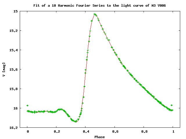