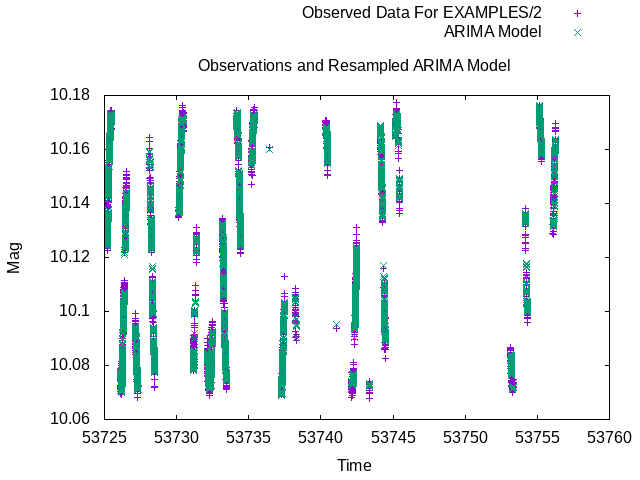
Fig 1. Comparison of observations and re-sampled ARIMA model produced in Example 3 for the sinusoidally variable light curve EXAMPLES/2.
Syntax:
-R
    < "fromfile" commandfile | commandstring >
    ["init" <"file" initializationfile | initializationstring>
        | "continueprocess" prior_R_command_number]
    ["vars" variablelist
        | ["invars" inputvariablelist] ["outvars" outputvariablelist]]
    ["outputcolumns" variablelist] ["process_all_lcs"]
Example 1.
$ ./vartools -l EXAMPLES/lc_list \
             -inputlcformat t:1,mag:2,err:3 \
             -header \
             -R 'b <- sd(mag)' \
                 invars mag outvars b outputcolumns b

#Name R_b_0
EXAMPLES/1 0.15946976931434592
EXAMPLES/2 0.036640196913116818
EXAMPLES/3 0.0048962905656505422
EXAMPLES/4 0.0020915710522042882
EXAMPLES/5 0.002880850234933455
EXAMPLES/6 0.0020898736803245783
EXAMPLES/7 0.003488095003079855
EXAMPLES/8 0.0022502571019889705
EXAMPLES/9 0.0018673694762206033
EXAMPLES/10 0.0023627959129451301
Example of using R to calculate the standard deviation in the magnitudes for each light curve read from the list file EXAMPLES/lc_list. The R expression "b <- sd(mag)" will be evaluated for each light curve. The variable "mag" will be passed as an input to the R command (it will be treated within R as a numeric vector of length equal to the number of observations), and the variable "b" will be read out from the command. The value of this variable, which stores the standard deviation, will be included as a column in the output ASCII table.
Example 2.
$ ./vartools -l EXAMPLES/lc_list \
             -inputlcformat t:1,mag:2,err:3 \
             -header \
             -R 'b <- list();
                 for(i in 1:length(mag)) {
                    b[[i]] <- sd(mag[[i]]);
                 }' \
                 invars mag outvars b outputcolumns b process_all_lcs

#Name R_b_0
EXAMPLES/1 0.15946976931434592
EXAMPLES/2 0.036640196913116818
EXAMPLES/3 0.0048962905656505422
EXAMPLES/4 0.0020915710522042882
EXAMPLES/5 0.002880850234933455
EXAMPLES/6 0.0020898736803245783
EXAMPLES/7 0.003488095003079855
EXAMPLES/8 0.0022502571019889705
EXAMPLES/9 0.0018673694762206033
EXAMPLES/10 0.0023627959129451301
Same as example 1, in this case we use the "process_all_lcs" keyword to send all of the light curve data to R at once. In this case the input light curve vectors will be made available as lists of vectors in R, where the Nth element in the list for a variable (e.g., mag) corresponds to that vector for light curve N. The output variable b in this case needs to be a list, with the Nth element in the list corresponding to the computed value for light curve N.
Example 3.
$ vartools -l EXAMPLES/lc_list \
    -inputlcformat t:1,mag:2,err:3 \
    -header \
    -savelc \
    -binlc average binsize 0.05 taverage \
    -resample linear delt fix 0.05 \
    -R \
       'mag_ts <- ts(mag, start=1, end=length(mag), frequency=1);
          arima_model <- auto.arima(mag_ts);
          mag_arima <- mag - as.vector(arima_model$residuals);' \
       init 'library(tseries); library(forecast);' \
       invars mag outvars mag_arima \
    -resample linear file list listcolumn 1 tcolumn 1 \
    -restorelc 1 vars mag \
    -o EXAMPLES/OUTDIR1 nameformat '%s.arimamodel' \
       columnformat t,mag,mag_arima \
  2> /dev/null

#Name
EXAMPLES/1
EXAMPLES/2
EXAMPLES/3
EXAMPLES/4
EXAMPLES/5
EXAMPLES/6
EXAMPLES/7
EXAMPLES/8
EXAMPLES/9
EXAMPLES/10

$ head -3 EXAMPLES/OUTDIR1/1.arimamodel
53725.173920000001 10.085000000000001 10.069214881731755
53725.17654 10.0847 10.070167733349381
53725.17772 10.0825 10.070596880260995
In this example we use the forecast package in R to perform an ARIMA modelling of the light curves in the list file EXAMPLES/lc_list. Note that this is not meant to illustrate a suggested way to process the light curves (among other problems, ARIMA should not be applied to non-stationary data, like some of the light curves being processed here), but is meant simply to illustrate the use of the -R command in vartools. To run this example you would first need to install the tseries and forecast packages in R, which you can do by running install.packages("tseries") and install.packages("forecast") from within the R interpreter. After reading in the light curve, we issue the -savelc command to save a copy of the input mag vector, which we will want to recover later in the process. ARIMA works on evenly sampled data, so we first bin the light curves in time with the -binlc command, using average binning with a binsize of 0.05 days. We then use the -resample command to resample the light curves onto a uniform time grid (needed to fill in any missing time bins). In the call to R we will input the light curve vector mag and output the light curve vector mag_arima, which is created by the R command. The processing command creates a tseries object called mag_ts from the vector mag, which is needed as input to the next routine, auto.arima, which performs the ARIMA modeling, returning the fit object to arima_model. The last command extracts the model residuals from the arima_model object into a vector which is subtracted from the mag vector, with the results stored into the vector mag_arima. This now contains the ARIMA model light curve values. We use the init term to load the tseries and forecast libraries in R before processing any light curves. The following -resample command resamples the light curve and ARIMA model back onto the original time-base of the light curve using linear interpolation. We then use the -restorelc command to restore the mag vector only to its original form at the first -savelc command. The light curves, containing the columns t, mag and mag_arima are finally output to the directory EXAMPLES/OUTDIR1 with the suffix .arimamodel appended to the name of each light curve. We show the format for one of these light curves at the bottom of the example. The expression 2>/dev/null at the end of the command is used to suppress stderr, which in this case would include a variety of output from R (such as notifications that the libraries are loaded) that is all re-directed to stderr by VARTOOLS.
Fig 1. Comparison of observations and re-sampled ARIMA model produced in Example 3 for the sinusoidally variable light curve EXAMPLES/2.
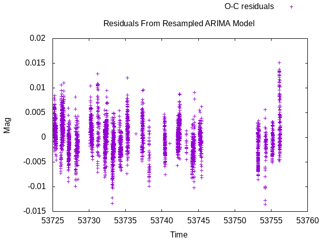
Fig 2. Residuals from ARIMA model for EXAMPLES/2 produced in Example 3.
$ cat EXAMPLES/Rexample4.R

library(tseries)
library(forecast)

DoArimaFitPlot <- function(mag, plotoutdir, lcbasename) {
    mag_ts <- ts(mag, start=1, end=length(mag), frequency=1)
    arima_model <- auto.arima(mag_ts)
    mag_arima <- mag - as.vector(arima_model$residuals)
    mag_forecast <- forecast(arima_model)
    png(paste(plotoutdir, lcbasename, ".arimaforecast.png", sep=""), width=640, height=480)
    plot(mag_forecast)
    dev.off()
    png(paste(plotoutdir, lcbasename, ".arimaresiduals.png", sep=""), width=640, height=480)
    checkresiduals(arima_model)
    dev.off()
    return(mag_arima)
}

$ vartools -l EXAMPLES/lc_list \
    -inputlcformat t:1,mag:2,err:3 \
    -header \
    -savelc \
    -binlc average binsize 0.05 taverage \
    -resample linear delt fix 0.05 \
    -python 'lcbasename = Name.split("/")[-1]' \
        invars Name outvars lcbasename \
    -R 'mag_arima <- DoArimaFitPlot(mag, "EXAMPLES/OUTDIR1/", lcbasename)' \
        init file EXAMPLES/Rexample4.R \
        invars mag,t,lcbasename outvars mag_arima \
    -resample linear file list listcolumn 1 tcolumn 1 \
    -restorelc 1 vars mag \
    -o EXAMPLES/OUTDIR1 nameformat '%s.arimamodel' \
        columnformat t,mag,mag_arima \
  2> > /dev/null

#Name
EXAMPLES/1
EXAMPLES/2
EXAMPLES/3
EXAMPLES/4
EXAMPLES/5
EXAMPLES/6
EXAMPLES/7
EXAMPLES/8
EXAMPLES/9
EXAMPLES/10
Similar to Example 3, in this case we source the initialization code from the file EXAMPLES/Rexample4.R. In this file we also define a function DoArimaFitPlot which carries out the ARIMA modeling, and also creates .png plots showing the future forecast and residuals from the model. In our call to the -R command we then apply this function to each light curve. We use the call to -python to get the basename for the light curves (i.e., the name of the file with the leading directories stripped off) which will be stored in the variable lcbasename. This could be done within the call to -R as well, but here we illustrate the ability to mix calls to these different languages so that we can take advantage of the easy string handling in python and the analysis capabilities of R. The rest of the command proceeds as in Example 3. In this case the output includes the additional plots EXAMPLES/OUTDIR1/*.arimaforecast.png and EXAMPLES/OUTDIR1/*.arimaresiduals.png.
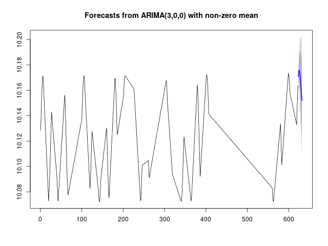
Fig 3. Plot EXAMPLES/OUTDIR2/2.arimaforecast.png produced by the call to DoArimaFitPlot for the light curve EXAMPLES/2 in Example 4.
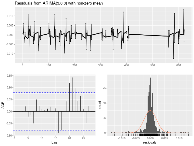
Fig 4. Plot EXAMPLES/OUTDIR2/2.arimaresiduals.png produced by the call to DoArimaFitPlot for the light curve EXAMPLES/2 in Example 4.