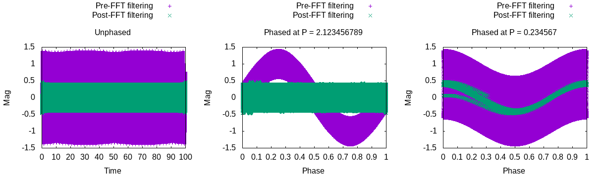
Fig 1. Light curve from Example 1 before and after applying the high-pass Fourier Filter.
Syntax:
-IFFT input_real_var input_imag_var output_real_var output_imag_var Example 1.
$ ./vartools -i EXAMPLES/11 \
    -FFT mag NULL fftreal fftimag \
    -rms \
    -expr \
      'fftreal=(NR>(Npoints_1/500.0))*(NR<(Npoints_1*499.0/500.0))*fftreal' \
    -expr \
      'fftimag=(NR>(Npoints_1/500.0))*(NR<(Npoints_1*499.0/500.0))*fftimag' \
    -IFFT fftreal fftimag mag_filter NULL \
    -o EXAMPLES/11.highpassfftfilter columnformat t,mag_filter

EXAMPLES/11   0.00070   0.76113   0.00100 100000
Example of using the -FFT and -IFFT commands to perform a high-pass Fourier-Filtering of a uniformly sampled time-series. The file EXAMPLES/11 is an idealized light curve containing 100,000 points at a uniform time-sampling of 0.001 days. The light curve is noise-free and contains the sum of two sinusoid signals, one with a period of 2.123456789 days and a semi-amplitude of 1.0, and the other with a period of 0.234567 days and a semi-amplitude of 0.4. This light curve is read into VARTOOLS, the -FFT command is called to calculate the Fourier transform of the 'mag' variable (assuming no imaginary component) and storing the real and imaginary components of the output transform in the fftreal and fftimag variables, respectively. The -rms command is used to determine the number of points in the time-series (stored in the variable Npoints_1 in this instance), and then the -expr commands are used to set the terms of the transform at frequencies |f|< 1.0/(500*0.001) to zero. The inverse transform is then applied to the filtered fftreal and fftimag variables, with the real output being stored in mag_filter and the imaginary output being ignored. The resulting high-pass filtered light curve is then output to the file EXAMPLES/11.highpassfftfilter.
Fig 1. Light curve from Example 1 before and after applying the high-pass Fourier Filter.
$ ./vartools -i EXAMPLES/2 \
    -resample splinemonotonic gaps percentile_sep 80 bspline \
    -FFT mag NULL fftreal fftimag \
    -rms \
    -expr 'fftreal1=(NR>(Npoints_2/10.0))*(NR<(Npoints_2*9.0/10.0))*fftreal' \
    -expr 'fftimag1=(NR>(Npoints_2/10.0))*(NR<(Npoints_2*9.0/10.0))*fftimag' \
    -IFFT fftreal1 fftimag1 mag_filter NULL \
    -expr 'fftreal2=fftreal-((NR>(Npoints_2/10.0))*(NR<(Npoints_2*9.0/10.0))*fftreal)' \
    -expr 'fftimag2=fftimag-((NR>(Npoints_2/10.0))*(NR<(Npoints_2*9.0/10.0))*fftimag)' \
    -IFFT fftreal2 fftimag2 mag_filter2 NULL \
    -resample linear file fix EXAMPLES/2 column 1 \
    -expr 'mag_filter=mag_filter+Mean_Mag_2' \
    -o EXAMPLES/2.fftfilter columnformat t,mag_filter,mag_filter2,mag

EXAMPLES/2  10.11155   0.02901   0.00028 66186
Similar to Example 1, here we apply the transform, filter, and inverse transform to a light curve with noise and non-uniform time-sampling. The -resample commands in this case are used to sample the light curve onto a uniform time-grid, and then to resample it back onto the original time-grid after applying the inverse transform. Here we store both the high-pass and low-pass filtered data. The filtering is much less effective in this non-idealized case where the original light curve has highly non-uniform sampling characteristic of single-site ground-based data obtained over multiple nights.
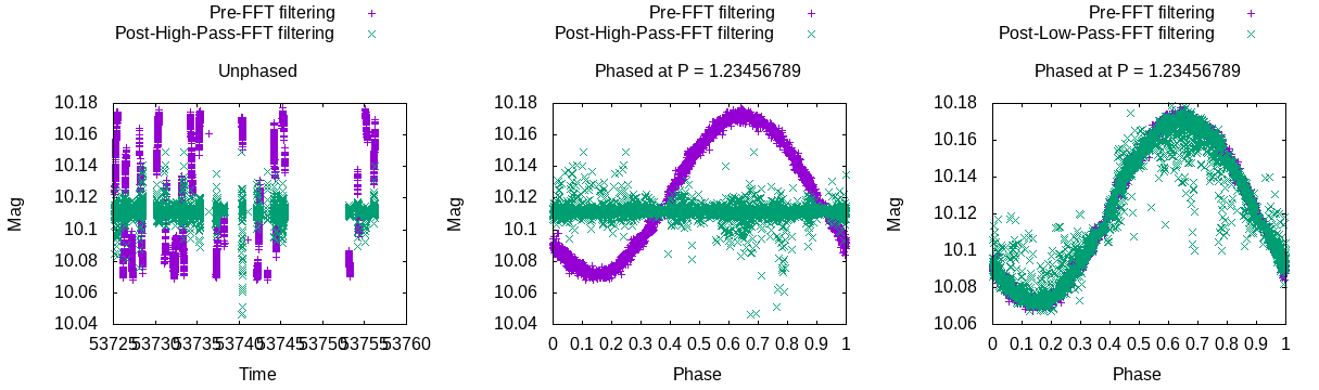
Fig 2. Light curve from Example 2 before and after applying the high-pass and low-pass Fourier Filters.