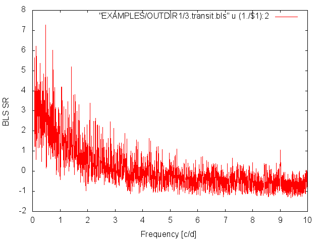
Fig 1. BLS spectrum computed in Example 1.
Syntax:
-BLS < "r" rmin rmax | "q" qmin qmax > minper maxper nfreq nbins timezone Npeak outperiodogram [outdir] omodel [model_outdir] correctlc ["fittrap"] ["nobinnedrms"] ["ophcurve" outdir phmin phmax phstep] ["ojdcurve" outdir jdstep] Example 1.
$ ./vartools -i EXAMPLES/3.transit -ascii -oneline \
    -BLS q 0.01 0.1 0.1 20.0 100000 200 0 1 \
        1 EXAMPLES/OUTDIR1/ 1 EXAMPLES/OUTDIR1/ 0 fittrap \
        nobinnedrms ophcurve EXAMPLES/OUTDIR1/ -0.1 1.1 0.001

Name                         = EXAMPLES/3.transit
BLS_Period_1_0               =     2.12334706
BLS_Tc_1_0                   = 53727.297293937358
BLS_SN_1_0                   =   7.26127
BLS_SR_1_0                   =   0.00238
BLS_SDE_1_0                  =   6.34195
BLS_Depth_1_0                =   0.01220
BLS_Qtran_1_0                =   0.03576
BLS_Qingress_1_0             =   0.19618
BLS_OOTmag_1_0               =  10.16686
BLS_i1_1_0                   =   0.98213
BLS_i2_1_0                   =   1.01790
BLS_deltaChi2_1_0            = -24217.21939
BLS_fraconenight_1_0         =   0.43155
BLS_Npointsintransit_1_0     =   165
BLS_Ntransits_1_0            =     4
BLS_Npointsbeforetransit_1_0 =   127
BLS_Npointsaftertransit_1_0  =   143
BLS_Rednoise_1_0             =   0.00151
BLS_Whitenoise_1_0           =   0.00489
BLS_SignaltoPinknoise_1_0    =  14.38935
BLS_Period_invtransit_0      =     1.14594782
BLS_deltaChi2_invtransit_0   = -3301.69183
BLS_MeanMag_0                =  10.16740
Apply the Box-Least Squares (BLS) transit-search algorithm to the light curve EXAMPLES/3.transit (an LC with a transit injected). At each trial frequency we scan fractional transit durations between 0.01 and 0.1 (the option q fixes the range, if we had used r then the range of transit durations to search would depend on the trial frequency). Periods between 0.1 and 20.0 days are searched. A total of 100000 frequencies are searched, and at each frequency we use 200 phase-bins. The time-zone is set to 0 (this only affects how the BLS_fraconenight output statistic is calculated). We only search for one peak in the BLS spectrum. The BLS spectrum is output to the directory EXAMPLES/OUTDIR1 (the -ascii option causes this to be written as an ascii file rather than the default binary file format), with the filename 3.transit.bls. The best-fit box-transit model is written to the directory EXAMPLES/OUTDIR1 with the filename 3.transit.bls.model. We do not subtract the best-fit transit before passing to the next command (in this example there are no further commands). By specifying fittrap we have the routine fit a trapezoid-shaped transit model after finding the top peak in the BLS spectrum. By specifying nobinnedrms we speed up the routine compared to the default behavior. We output a model transit phase curve to EXAMPLES/OUTDIR1/ (it will have the filename 3.transit.bls.phcurve), this can be used for overplotting the model on the data in the file bls.model (which is only sampled at the observed phases). The phase curve will go from -0.1 to 1.1 with a step-size of 0.001 in phase. By giving the -oneline option before the -BLS command we have the statistics written with one line per statistic.
Fig 1. BLS spectrum computed in Example 1.
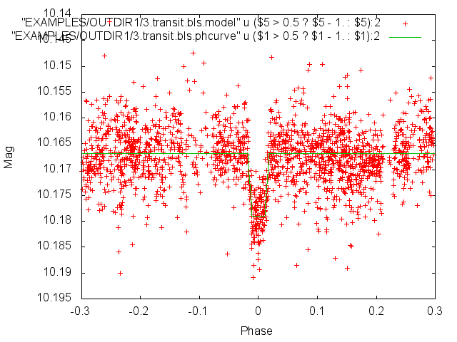
Fig 2. Phased transit light curve and BLS model from Example 1.