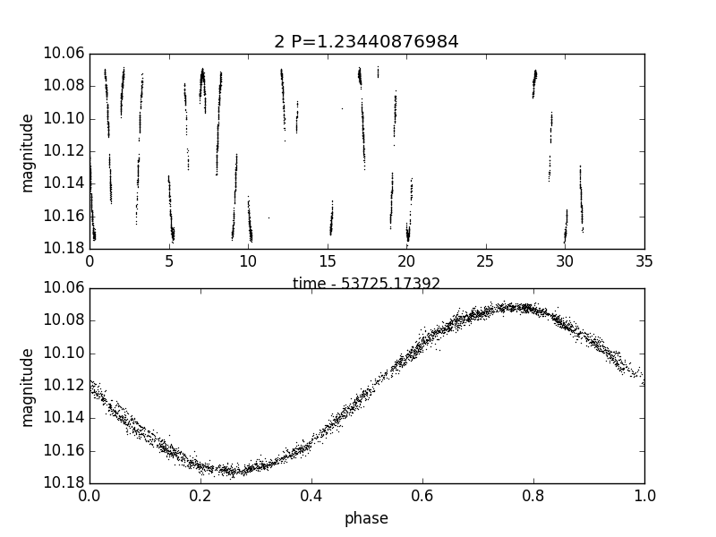
Fig 1. Plot EXAMPLES/2.png produced by the call to plotlc for the light curve EXAMPLES/2 in Example 2.
Syntax:
-python
    < "fromfile" commandfile | commandstring >
    ["init" <"file" initializationfile | initializationstring>
        | "continueprocess" prior_python_command_number]
    ["vars" variablelist
        | ["invars" inputvariablelist] ["outvars" outputvariablelist]]
    ["outputcolumns" variablelist] ["process_all_lcs"]
Example 1.
$ ./vartools -l EXAMPLES/lc_list \
             -inputlcformat t:1,mag:2,err:3 \
             -header \
             -python 'b = numpy.var(mag)' \
                      invars mag outvars b outputcolumns b

#Name PYTHON_b_0
EXAMPLES/1 0.025422461711037084
EXAMPLES/2 0.0013420988067623005
EXAMPLES/3 2.3966645306408949e-05
EXAMPLES/4 4.3733138204733634e-06
EXAMPLES/5 8.2971716866526236e-06
EXAMPLES/6 4.3664615059428104e-06
EXAMPLES/7 1.216345131566495e-05
EXAMPLES/8 5.0623773543353351e-06
EXAMPLES/9 3.4861868515750583e-06
EXAMPLES/10 5.5813996936871234e-06
Example of using python to calculate the variance in the magnitudes for each light curve read from the list file EXAMPLES/lc_list. The python expression "b = numpy.var(mag)" will be evaluated for each light curve. The variable "mag" will be passed as an input to the python command (it will be treated as a numpy array within python), and the variable "b" will be read out from the command. The value of this variable, which stores the variance, will be included as a column in the output ASCII table.
Example 2.
$ cat EXAMPLES/plotlc.py

import matplotlib.pyplot as plt

def plotlc(lcname,outdir,t,ph,mag,P):
    lcbasename = lcname.split('/')[-1]
    plt.figure(1)
    plt.subplot(211)
    plt.gca().invert_yaxis()
    tcorr = t - t[0]
    plt.plot(tcorr, mag, 'bo', markersize=0.5)
    plt.ylabel('magnitude')
    plt.title(lcbasename+' P='+str(P))
    plt.xlabel('time - '+str(t[0]))
    plt.subplot(212)
    plt.gca().invert_yaxis()
    plt.plot(ph, mag, 'bo', markersize=0.5)
    plt.ylabel('magnitude')
    plt.xlabel('phase')
    plt.savefig(outdir+'/'+lcbasename+'.png',format="png")
    plt.close()

$ vartools -l EXAMPLES/lc_list -inputlcformat t:1,mag:2,err:3 -header \
    -LS 0.1 100. 0.1 1 0 \
    -if 'Log10_LS_Prob_1_0<-100' \
        -Phase ls phasevar ph \
        -python 'plotlc(Name,"EXAMPLES/",t,ph,mag,LS_Period_1_0)' \
            init file EXAMPLES/plotlc.py \
    -fi

#Name LS_Period_1_0 Log10_LS_Prob_1_0 LS_Periodogram_Value_1_0 LS_SNR_1_0
EXAMPLES/1    77.76775250 -5710.91013    0.99392   38.81513
EXAMPLES/2     1.23440877 -4000.59209    0.99619   45.98308
EXAMPLES/3    18.29829471  -26.09202    0.03822   11.87999
EXAMPLES/4     0.99383709  -90.59677    0.12488   11.63276
EXAMPLES/5     7.06979568  -86.82830    0.10042   11.03518
EXAMPLES/6    22.21935786  -59.44675    0.07034    9.96198
EXAMPLES/7     0.14747089  -12.56404    0.01933    4.85468
EXAMPLES/8     0.93696087  -79.26500    0.09115    9.35161
EXAMPLES/9     7.06979568  -48.29326    0.05781   11.13720
EXAMPLES/10     0.96906857  -52.91818    0.06257    9.66926
Example of running the Lomb-Scargle periodogram on light curves in the list file EXAMPLES/lc_list, and then using matplotlib.pyplot in python to create .png plots of those light curves which have a log10 false alarm probability from LS of less than -100. The routine for plotting a light curve is stored in the file EXAMPLES/plotlc.py, where we import the matplotlib.pyplot module and then define a python function for making a plot. We use the "init file" option to the -python command in VARTOOLS to load this code on initialization (technically the code is incorporated into a module together with a function that VARTOOLS constructs for calling the python commands to be run on each light curve). The expression 'plotlc(Name,"EXAMPLES/",t,ph,mag,LS_Period_1_0)' will then be executed on each light curve, where the variable "Name" stores the full light curve name, "ph" stores the phases which are calculated with the -Phase command, and "LS_Period_1_0" is the period returned by the -LS command.
When run on the files in EXAMPLES/lc_list this will produce the plots EXAMPLES/1.png and EXAMPLES/2.png showing the light curves vs time and phase.
Note that to run this example vartools will need to be compiled against a version of python which is able to import matplotlib.
Fig 1. Plot EXAMPLES/2.png produced by the call to plotlc for the light curve EXAMPLES/2 in Example 2.
$ vartools -l EXAMPLES/lc_list -inputlcformat t:1,mag:2,err:3 -header \
    -LS 0.1 100. 0.1 1 0 \
    -Phase ls phasevar ph \
    -python \
        'for i in range(0,len(mag)):
            plotlc(Name[i],"EXAMPLES/",t[i],ph[i],mag[i],LS_Period_1_0[i])' \
        init file EXAMPLES/plotlc.py \
        process_all_lcs

#Name LS_Period_1_0 Log10_LS_Prob_1_0 LS_Periodogram_Value_1_0 LS_SNR_1_0
EXAMPLES/1    77.76775250 -5710.91013    0.99392   38.81513
EXAMPLES/2     1.23440877 -4000.59209    0.99619   45.98308
EXAMPLES/3    18.29829471  -26.09202    0.03822   11.87999
EXAMPLES/4     0.99383709  -90.59677    0.12488   11.63276
EXAMPLES/5     7.06979568  -86.82830    0.10042   11.03518
EXAMPLES/6    22.21935786  -59.44675    0.07034    9.96198
EXAMPLES/7     0.14747089  -12.56404    0.01933    4.85468
EXAMPLES/8     0.93696087  -79.26500    0.09115    9.35161
EXAMPLES/9     7.06979568  -48.29326    0.05781   11.13720
EXAMPLES/10     0.96906857  -52.91818    0.06257    9.66926
Same as in example 2, except here we plot all of the light curves (no -if command to VARTOOLS), and we use the process_all_lcs keyword to send all of the light curves to python at once. In this case VARTOOLS supplies these as lists of numpy arrays, so we use the for loop to cycle through all of the light curves calling plotlc on each light curve in turn.