
Fig 1. DFT Power Spectrum computed in Example 1.
Syntax:
-dftclean nbeam ["maxfreq maxf"] ["outdspec" dspec_outdir] ["finddirtypeaks" Npeaks ["clip" clip clipiter]] ["outwfunc" wfunc_outdir] ["clean" gain SNlimit ["outcbeam" cbeam_outdir] ["outcspec" cspec_outdir] ["findcleanpeaks" Npeaks ["clip" clip clipiter]]] ["useampspec"] ["verboseout"] Example 1.
$ ./vartools -i EXAMPLES/2 -oneline -ascii \
    -dftclean 4 maxfreq 10. outdspec EXAMPLES/OUTDIR1 \
        finddirtypeaks 1 clip 5. 1

Name                         = EXAMPLES/2
DFTCLEAN_DSPEC_PEAK_FREQ_0_0 =     0.81189711
DFTCLEAN_DSPEC_PEAK_POW_0_0  = 0.000687634
DFTCLEAN_DSPEC_PEAK_SNR_0_0  =   59.8532
Compute the Discrete Fourier Transform (DFT) of the light curve EXAMPLES/2. We will over-sample the DFT by a factor of 4, and compute the DFT up to a maximum frequency of 10 cycles per day. The resulting power spectrum will be output to the directory EXAMPLES/OUTDIR1 with the filename 4.dftclean.dspec. We search for the highest peak in the power spectrum using a 5-sigma iterative clipping to determine the spectroscopic signal-to-noise ratio of the peak. In this example the highest peak is at 0.81189711 cycles/day corresponding to a period of 1.23168 days, which is close to the injected period of 1.2354 days.
Fig 1. DFT Power Spectrum computed in Example 1.
$ ./vartools -i EXAMPLES/4 -oneline -ascii \
    -Injectharm fix 0.697516 0 ampfix 0.1 phaserand 0 0 \
    -Injectharm fix 2.123456 0 ampfix 0.05 phaserand 0 0 \
    -Injectharm fix 0.426515 0 ampfix 0.01 phaserand 0 0 \
    -dftclean 4 maxfreq 10. outdspec EXAMPLES/OUTDIR1 \
        finddirtypeaks 3 clip 5. 1 \
        outwfunc EXAMPLES/OUTDIR1 \
        clean 0.5 5.0 outcbeam EXAMPLES/OUTDIR1 \
        outcspec EXAMPLES/OUTDIR1 \
        findcleanpeaks 3 clip 5. 1 \
        verboseout

Name                            = EXAMPLES/4
Injectharm_Period_0             =     0.69751600
Injectharm_Fundamental_Amp_0    =   0.10000
Injectharm_Fundamental_Phase_0  =   0.84019
Injectharm_Period_1             =     2.12345600
Injectharm_Fundamental_Amp_1    =   0.05000
Injectharm_Fundamental_Phase_1  =   0.39438
Injectharm_Period_2             =     0.42651500
Injectharm_Fundamental_Amp_2    =   0.01000
Injectharm_Fundamental_Phase_2  =   0.78310
DFTCLEAN_DSPEC_PEAK_FREQ_0_3    =     1.43890675
DFTCLEAN_DSPEC_PEAK_POW_0_3     = 0.0033349
DFTCLEAN_DSPEC_PEAK_SNR_0_3     =    67.932
DFTCLEAN_DSPEC_PEAK_FREQ_1_3    =     0.43408360
DFTCLEAN_DSPEC_PEAK_POW_1_3     = 0.00294915
DFTCLEAN_DSPEC_PEAK_SNR_1_3     =   59.9866
DFTCLEAN_DSPEC_PEAK_FREQ_2_3    =     2.43569132
DFTCLEAN_DSPEC_PEAK_POW_2_3     = 0.00209661
DFTCLEAN_DSPEC_PEAK_SNR_2_3     =   42.4262
DFTCLEAN_DSPEC_AVESPEC_3        = 3.68371e-05
DFTCLEAN_DSPEC_STDSPEC_3        = 4.85494e-05
DFTCLEAN_DSPEC_AVESPEC_NOCLIP_3 = 8.70341e-05
DFTCLEAN_DSPEC_STDSPEC_NOCLIP_3 = 0.000277645
DFTCLEAN_CSPEC_PEAK_FREQ_0_3    =     1.43086817
DFTCLEAN_CSPEC_PEAK_POW_0_3     = 0.00295622
DFTCLEAN_CSPEC_PEAK_SNR_0_3     =      8650
DFTCLEAN_CSPEC_PEAK_FREQ_1_3    =     0.47427653
DFTCLEAN_CSPEC_PEAK_POW_1_3     = 0.000488863
DFTCLEAN_CSPEC_PEAK_SNR_1_3     =   1429.81
DFTCLEAN_CSPEC_PEAK_FREQ_2_3    =     2.34726688
DFTCLEAN_CSPEC_PEAK_POW_2_3     = 2.55442e-05
DFTCLEAN_CSPEC_PEAK_SNR_2_3     =   74.0001
DFTCLEAN_CSPEC_AVESPEC_3        = 3.41729e-07
DFTCLEAN_CSPEC_STDSPEC_3        = 2.56197e-07
DFTCLEAN_CSPEC_AVESPEC_NOCLIP_3 = 0.000309941
DFTCLEAN_CSPEC_STDSPEC_NOCLIP_3 = 5.52828e-05
A slightly more involved example to illustrate the use of the clean algorithm. Here 3 harmonic signals are added to the light curve EXAMPLES/4 with periods of 0.697516, 2.123456 and 0.426515 days, and amplitudes of 0.1, 0.05 and 0.01 mag. We then calculate the DFT as in Example 1, but this time we determine the 3 highest peaks in the DFT and we also output the window function to EXAMPLES/OUTDIR1 (the filename will be 4.dftclean.wfunc). We then apply the CLEAN deconvolution algorithm to the DFT using a gain of 0.5 and a S/N threshold of 5.0. The clean-beam, and clean power spectrum are written to EXAMPLES/OUTDIR1 (with filenames 4.dftclean.cbeam and 4.dftclean.cspec respectively). We search the clean power spectrum for 3 peaks, and include the average and standard deviation of the dirty and clean power spectra in the output table of statistics. The frequencies found in the clean spectrum are a little closer to the injected frequencies.

Fig 2. DFT Power Spectrum computed in Example 2.
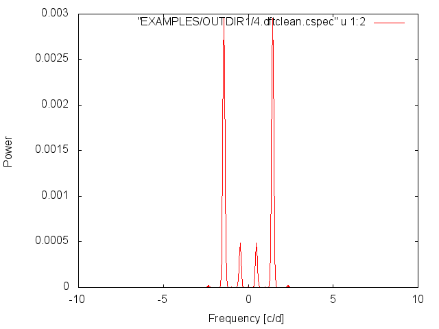
Fig 3. DFT Power Spectrum after application of CLEAN deconvolution from Example 2.
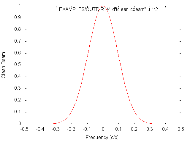
Fig 4. Clean Beam for Example 2.
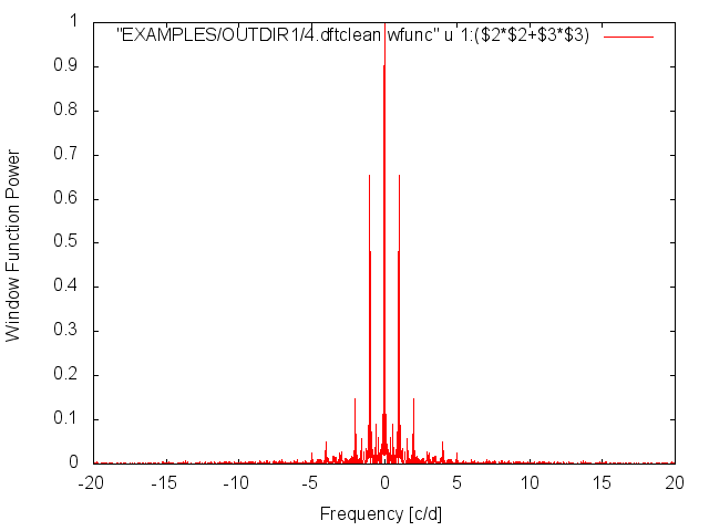
Fig 5. Window Function for Example 2.