The scientific returns of the imaging survey depend to a large extent on the accuracy of its photometric calibration. A 10-Terabyte multiband data set that covers pi steradians of the sky, in which there are 108 sources bright enough to be well measured, can be used to investigate exceedingly subtle phenomena, provided the photometry is adequate. The fundamental issue of the isotropy of the galaxy distribution over large angles depends in an essential way on how well the photometric zero point has been transferred across the sky, and on the proper evaluation of Galactic absorption. For example, Burstein and Heiles (1978, 1982) estimate the errors in their reddening maps to be at the level of delta E(B-V)=0.03 ; this variation alone would result in an error in the galaxy surface density of about 14%.
The photometric accuracy is driven by three science requirements:
1. QSO Photometry: Experience with using existing color data to separate stars and QSOs is that systematic photometric errors in the colors should be no larger than about 5%.
2. Large-scale structure studies: Imagine scanning a single strip for the entire night(2.5° by 120°). The most demanding analysis that one can do is to divide the strip into two halves and measure the difference in galaxy counts between the two. For the spectroscopic sample (magnitude limit about 18 in r' ), the rms scatter in this difference due to the known large scale clustering is expected to be at least 8%. The rms systematic photometric error should therefore be no larger than half of this, or 4% in galaxy counts; using a value of 0.5 for d log N/dm , this corresponds to a 3% rms error in photometry in the band used to select the galaxies. If we repeat the exercise for ALL galaxies identified by the imaging survey (which reaches much fainter than 20m ), the fluctuations due to clustering will be much weaker, perhaps less than 1%. Thus, we could make use of data with systematic errors smaller than 0.5% rms.
3. Interstellar reddening: The ultimate limit in analyzing galaxy counts is set by fluctuations in the interstellar reddening and extinction. The primary technique used to find the extinction is to measure the shifts in color of some class of objects and to use standard conversions from selective to total extinction. From published Gunn-Thuan photometry (Thuan and Gunn 1976; Schneider, Gunn and Hoessel 1983), we find that Ar = 2.1 Eg-r , so that the colors must be measured twice as accurately as the desired accuracy of the extinction itself. Calibration of the Galactic extinction thus requires that color errors be less than about 1.5% rms for the analysis of the spectroscopic sample and 0.25% for the full imaging sample.
Regardless of the science one is trying to do, the limiting accuracy to which reddening and extinction can be measured is ultimately set by irreducible systematic errors in the technique used to measure the reddening. If we did nothing beyond using the Burstein-Heiles extinction map we would not be able to extract the full amount of information available in the imaging survey. We expect to investigate several techniques to improve on the existing reddening maps but the limiting accuracy is not knowable in advance. For example, one promising technique is to measure the g' - r' color distribution of stars at around magnitude 18; the halo stars form a strongly peaked distribution whose width is about 0.3 magnitudes and whose centroid can be measured to perhaps 0.03 magnitudes. The position of the peak will depend on both reddening and population variations (metallicity and age). If the latter effects can be calibrated, we will have a powerful technique for measuring the reddening. To do so with sufficient accuracy requires that the stellar colors should have systematic photometric errors of order 0.015 magnitudes.
After considering the above factors, we have set the requirements for the photometric calibration accuracy of the imaging survey to be no worse than 2% rms in magnitudes and colors averaged over degree sized areas, with a goal to achieve twice that accuracy.
Our requirement of 2% rms error ought to be easily achievable based on our and others experience with carrying out precision photometry. The limits to photometric accuracy are usually set by the accumulation of several small sources of error, each of comparable magnitude. Some of these are:
We will establish the primary photometric calibration for the survey by using a small robotic telescope at the 2.5-m survey telescope site. This instrument will observe continuously and automatically a set of photometric standards to calibrate the main survey.
The primary standard stars for the SDSS system are a grid of 20-30 bright, isolated stars in each of the northern and southern skies. All are photometric standards in current use, and a few have absolute calibrations. The energy distributions of these standard stars have been transferred to the SDSS filter system (Fukugita et al. 1996). A subset of the primary standards will be observed nightly by the Monitor Telescope, efficiently placing the survey telescope imaging data onto an absolute photometric system.
The telescope itself is a 0.61 m automatic telescope purchased commercially from the Autoscope Corporation. It is an f/10 Ritchey-Chrétien design with a Gascoigne corrector and field flattener to provide 0.6" images over a 40' diameter field of view. The telescope control system was supplied by Autoscope but it is being reworked for the survey. The data acquisition system hardware is provided by Fermilab. The camera is a slightly modified version of the spectroscopic camera electronics. The detector is a thinned Tektronix 2048 x 2048 CCD with 0.8" pixels and a 27' square field of view. The telescope and its dome will be capable of autonomous operation from a cold start for extended periods of time. The telescope and all instrumentation are installed at the site and have been undergoing commissioning tests for several months. Monitor telescope images of a standard star field are shown in Figure 5.1.
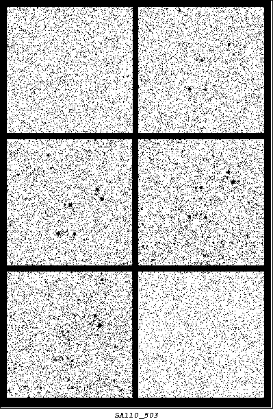
CCD images of the Landolt standard star field SAO110503. Five images were obtained with the monitor telescope in the SDSS u'g'r'i'z' filters. The sixth panel is intentionally left blank.
The Monitor Telescope will be used for several months in advance of the main Survey to observe extensively the primary standard star network and define the SDSS photometric system. During the survey, it will operate in parallel with the 2.5 m telescope, observing both primary standard stars and a set of secondary transfer fields that will be be scanned by the 2.5 m telescope. These data can be analyzed to provide the three necessary calibration coefficients needed to place the survey imaging data onto the SDSS photometric system.
The first coefficient is the atmospheric extinction. A minimum of 6 fundamental standard stars at a variety of airmasses will be observed each hour during the night in order to determine the extinction coefficients on an hourly basis.
The second coefficient is the photometric zeropoint for each 2.5 m photometric CCD. The Monitor Telescope will observe a grid of transfer star fields distributed throughout the SDSS survey area. We have selected a grid of 2392 fields, chosen to maximize the distance away from bright stars (see Figure 1.2). The Monitor Telescope observations calibrate the transfer fields so that when the main survey scans across them, we can use the known magnitudes in the fields to determine the zeropoints of the main survey photometry. Each transfer field must contain about 10 stars that do not saturate the SDSS camera but are measured with better than 1% accuracy rms by the Monitor Telescope. The zeropoints of the main survey may change with time because the field rotates with respect to the telescope pupil, so we will provide transfer fields for each scanline hourly. Each of the six scanlines will need its own transfer field. The Monitor Telescope will observe the transfer star field as nearly simultaneously with the main survey scan as feasible.
Last, there may be mismatches of the system efficiency as a function of wavelength between the main telescope and the Monitor Telescope because a single thinned Tektronix chip is used to calibrate all five bands (although the MT optics are coated to minimize this problem). This introduces color terms into the solutions. Experience has shown that such color terms change slowly with time (we will measure them once a week). The Monitor Telescope will observe secondary standard star patches known to contain a good distribution of star colors. Then, when convenient (for example, when there is some moonlight), all the CCDs in the SDSS camera will scan one of the color patches.
Second order coefficients (which account for the slight dependence of the atmospheric extinction on spectral energy distribution of a star or galaxy) will be included in the photometric solutions as well. We will try to measure them as well, although they are small enough that they can likely be computed in advance with sufficient accuracy.
A quick photometric solution will be computed in real time during the night. and provided to the observers conducting the main survey. This will allow them to monitor the quality of the night.
There are several special cases which need to be discussed. The u' band observations require special treatment as the stars that are bright enough to serve as standards in u' are saturated in the g'r'i' bands. We address this by allowing the random error to be higher in the u' band ( 2% instead of 1% ; this allows us to use fainter stars as standards) and by doubling the Monitor Telescope integration time on the the u' standards.
A second special case is the rapid variability in the near infrared sky, especially the water absorption bands. This will affect our ability to calibrate the i' and z' bands properly. We may choose to monitor the infrared sky on a nightly basis with two filters centered on the A band and an infrared H2O band. Observations through these filters will allow us to apply color terms due to the changing atmosphere to the photometric solution.
A third special case is the spectrophotometric calibration of the spectroscopic data. This will be accomplished by the use of 10 narrow-band filters, 8 spanning the wavelength range of the spectrograph, the other two to measure the A band and a suitable infrared water band, probably the same filters described in the last paragraph. The primary standard stars with absolute photometric calibrations will be observed with this filter set, and the system transferred to a set of secondary spectrophotometric standard stars, approximately three per spectroscopic field. These secondary stars in turn will be observed by the main survey spectrograph to provide the system response. The calibration of the secondary stars is an onerous task, but probably can be short-circuited. There are some tens of F subdwarfs per spectroscopic field which are sufficiently bright that high-quality spectra can be obtained. These stars are spectrophotometrically very similar, and the 5-color photometric data may be enough to determine the energy distribution to sufficient accuracy for flux calibration. We then need only to obtain 10 band photometry of a grid of such subdwarfs, which is a much smaller number than the total number of secondary spectroscopic standards.
The Monitor Telescope must be able to observe 6 bright standard stars and 6 SDSS transfer star fields per hour in order to keep up with the imaging survey and provide enough stars to calibrate the atmospheric extinction and monitor the atmospheric transmission quality. Because the field of view of the monitor telescope is large, it is possible to observe transfer fields for two adjacent scanlines of the SDSS with one Monitor Telescope field, doubling the number of stars per scanline and cutting the number of Monitor Telescope fields in half. The monitor camera CCD will have 2 corner readouts with digitization times of 15 µsec per pixel. The time budget is then as follows:
(1) Integration time of bright standard star field plus 5 sec for filter positioning and overhead - 15 sec/frame; 6 fields x 5 filters; 7.5 minutes total per hour.
(2) Readout of bright standard star field - (central 1024 2 only) - 32 sec/frame; 6 fields x 5 filters; 16 min total per hour.
(3) Integration time of transfer fields plus 5 sec for filter positioning and miscellaneous overhead - 60 sec per frame ( g'r'i'z' ), 115 sec per frame ( u' ); 3 fields x 5 filters; 17.8 min total per hour.
(4) Readout of transfer fields - 32 sec/frame; 3 fields x 5 filters; 8.0 min total per hour.
(5) Slew time: 1 minute/field; 9 fields; 9 minutes total per hour.
Total: 58 minutes per hour. This leaves us little margin for unexpected difficulties, but some of the timings above are pessimistic and all are well known with the exception of u' band exposure times.
There will be two adjunct systems to the Monitor Telescope. Both provide data on the quality of the night to the survey observers. The first is an IR all-sky scanner. This 10 µ linear array camera complements the Monitor Telescope by providing continuous all-sky images that are very effective at detecting clouds. The scanner has been built, tested, and is now in routine use at the 3.5 m telescope. It performs extremely well. The second system is a small weather station that monitors temperature, wind, pressure, and humidity. We will use it in making qualitative assessments of the SDSS data quality (e.g., does bad seeing correlate with wind direction, wind speed, rapid temperature variations, etc.).
Burstein, D., and Heiles, C.E., 1978, ApJ 225, 40.
Burstein, D., and Heiles, C.E. 1982, AJ 87, 1165.
Fukugita, M., Ichikawa, T., Gunn, J.E., Doi, M., Schneider, D.P., and Shimasaku, K, 1996, AJ 111, 1748.
Schneider, D.P., Gunn, J.E., and Hoessel, J.G. 1983, ApJ 264, 337.
Thuan, T.X., and Gunn, J.E. 1976, PASP 88, 543.