
We have carried out extensive efforts to simulate the data that will be produced by the SDSS. These simulations serve several interrelated purposes. First, they provide data that we can use to test the survey's data acquisition and reduction software. Second, they help us make informed decisions about survey strategy -- target selection criteria, geometry, scheduling, and so forth. Third, they offer qualitative and quantitative predictions about what the SDSS should see, under specified theoretical assumptions. Fourth, they provide an artificial database that we can use to develop and test methods that we will eventually use to extract scientific information from the survey itself. Because the survey test year is fast approaching, we have so far focused our attention on the first of these applications, testing survey software. Once the survey is underway, the fourth application will assume great importance, especially for large scale structure studies. We will use simulations like those described below to calibrate uncertainties and check for biases in our methods of analysis, and to test the ability of the analysis to distinguish theoretical models of the large scale structure.
There are a number of survey software tasks that require simulated data. Of course we want to test the software on real data as well, but the real data will not be available until the survey telescope is in operation, and it is in any case useful to have some test data for which the "right" answer is known in advance. At the most nitty-gritty level, we need simulated data to test the photometric reduction software, everything from flat-fielding the CCD images to classifying objects and selecting spectroscopic targets. For this purpose, we need artificial images with realistic numbers of objects, realistic magnitudes, colors, sizes, and profiles, realistic clustering, and realistic seeing, noise, and defects. In the end, we can test for any biases in the selection of spectroscopic targets by passing artificial catalogs through the complete data reduction pipeline and comparing the actual target list to the list of targets that would have been selected if the data reduction were perfect.
For many other tests, we need only simulated catalogs , i.e. lists of objects with photometric properties and positions on the sky. We will use such catalogs to help us decide the selection criteria for spectroscopic targets. For galaxies, we want to know how different choices of selection criteria will affect our ability to measure large scale structure, and for quasars we want to estimate the impact of stellar contamination on the target lists as a function of Galactic latitude and longitude. We will also use simulated catalogs to test the efficiency of the tiling software described in Chapter 12, and to study the effects of the minimum fiber spacing on our ability to sample galaxy clusters, groups, and binaries. The simulations also allow us to examine the possible impact of photometry errors and uncertainty in Galactic extinction on measurements of galaxy clustering.
We have designed a three-tier system for creating simulated data; we have implemented many parts of this system, and are continuing to add new elements and refine existing ones. The first tier creates artificial sky catalogs -- lists of objects with positions and photometric parameters. We use a large, cosmological N-body simulation to provide a clustered galaxy distribution, and the Bahcall-Soneira (1984) model of the Galaxy for star counts. The second tier turns the catalog for a specific patch of sky into artificial images in the survey filter bands. Spiral galaxies are represented by inclined exponential disks, elliptical galaxies and bulges by spheroids with a de Vaucouleurs-law profile, and stars and quasars by point sources. The images are convolved with a point-spread function (PSF), and noise and other artifacts (cosmic rays, diffraction spikes, etc.) are added, as are the defects of real CCDs (see below). The third tier of the simulation system turns a series of artificial images into a data stream that looks like it is coming from the telescope's data acquisition system. We can thus run simulated data all the way through the photometric data reduction pipeline. The next section describes the first tier of this system, sky catalogs, in greater detail. Section 9.2 describes the other two tiers, in particular our techniques for creating artificial images.
A complete simulated catalog would list positions and parameters of galaxies, stars, and quasars, about a magnitude deeper than the depth of the photometric survey, covering the whole SDSS footprint on the sky. Such a catalog would be rather unwieldy, and in practice we use programs to create either a photometric-depth catalog over a rather limited area of sky or a catalog over the whole survey region but only to the depth of the spectroscopic survey. It is nonetheless useful to think in terms of "the" catalog that in principle contains all of the objects that the survey might observe in a simulated universe. Our convention is that the catalogs list "intrinsic" apparent parameters, with no instrumental or atmospheric effects, the sort of numbers that we want our data reduction software to produce and store in the data archive.
Galaxies are the most challenging component of the artificial catalog, since we require a population of objects with realistic spatial clustering, luminosities, diameters, and colors. Trickier still, we need to include any important correlations between these properties, to the extent that they are known observationally. The basis of the galaxy catalog is a large N-body simulation run by Changbom Park and Richard Gott. The simulation uses Park's (1990) particle-mesh, N-body code to evolve 380³ ~ 55 million particles on a 600³ mesh that represents a comoving, periodic cube 600 h-1 Mpc on a side. The background cosmological model is a flat universe with Omega0=0.4, a cosmological constant Lambda0=0.6 , and a Hubble constant h=0.6 . The initial conditions are Gaussian fluctuations with a cold dark matter (CDM) power spectrum corresponding to these values of Omega0 and h . The normalization of the initial fluctuations corresponds to a "bias factor" of 1.3 in spheres of radius 8 h-1 Mpc , and "galaxies" are represented by a weakly biased subset of the full particle distribution, corresponding to nu >0.7 peaks of the initial density field, so that their clustering amplitude matches observations. The number density of the biased particles is sufficient to represent galaxies brighter than about 0.064 L*. There are just over 8 million galaxy particles in the simulation volume.
The logic behind using the CDM + Lambda model is simple: it produces a galaxy distribution whose clustering properties match existing observational data quite well over a wide range of scales. For the purpose of providing test data, the physical attractiveness or unattractiveness of the model is not particularly important -- we just want something that looks reasonably like the observed universe. To go from the distribution of particles in the N-body simulation to a galaxy catalog, we need to assign apparent fluxes and diameters in the survey bands, for an "observer" located in one corner of the simulation cube. Each galaxy particle is assigned an absolute blue (BT) luminosity drawn randomly from a Schechter luminosity function. The luminosity distribution is cut off below 0.064 L* (about 3 magnitudes below M*) in order to match the galaxy density of the simulation. Each galaxy is also assigned a randomly chosen Hubble type from E to Sc, with relative probabilities determined from the local galaxy density using the observed morphology-density relation in the form given by Postman & Geller (1984). The galaxy can then be assigned an apparent flux in each of the survey bands using the appropriate colors and K-corrections; these are computed for each Hubble type using Coleman et al.'s (1980) galaxy spectrophotometry and the filter-response curves illustrated in Figure 4.1. To assign diameters in accordance with the luminosity, we use a mean relation based on the fundamental plane (for ellipticals) and a Freeman law (for disks). We add scatter about these mean relations, so that our simulated catalog includes both low surface brightness galaxies and compact, high surface brightness galaxies.
The N-body simulation is large enough to contain almost the full galaxy redshift sample, without periodic replications. To reach the depth of the photometric sample, we must wrap around the periodic boundary several times. A random line of sight through the box is unlikely to pass near itself on later traversals, so this is not a serious problem.
For this example, we adopted an apparent magnitude limit of 17.55 in the r' band, and a minimum angular diameter (at the half-light radius) of 2 arcseconds (these simulations were done based on an earlier version of the target selection criteria). These limits yield just under a million galaxies over the survey region; about 2% of the galaxies brighter than the limiting magnitude are rejected because they are smaller than the imposed minimum diameter.
The upper panel of Figure 9.1 is a 6 degree by 130 degree redshift-space slice. The lower panel shows the same slice in real space, i.e. with peculiar velocities set to zero. The redshift-space slice clearly shows "fingers-of-God" caused by velocity dispersions in virialized groups and clusters. These thicken the extended filaments and sheets, making them more prominent.
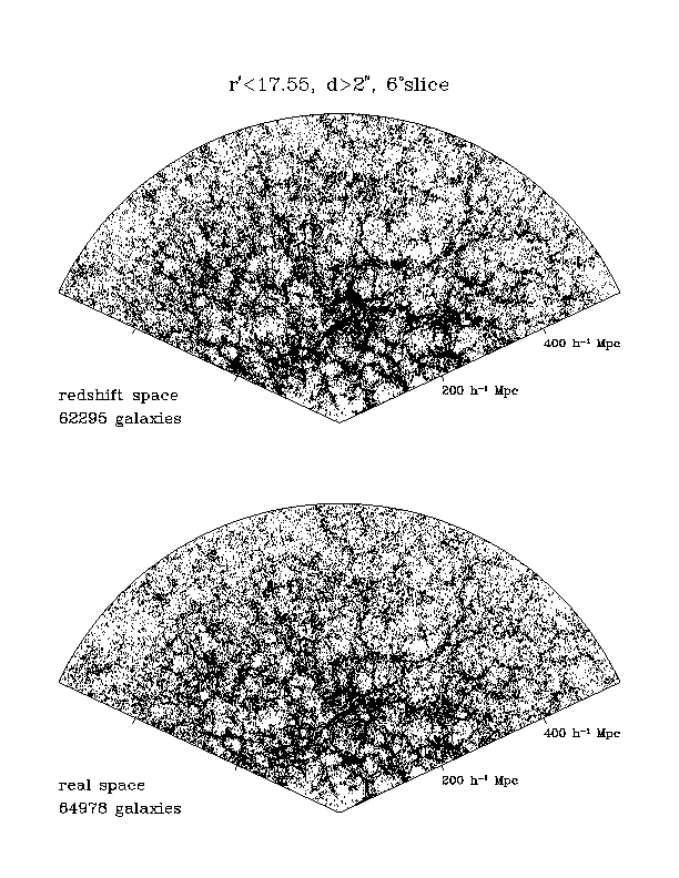
Slices from a simulation of the SDSS redshift survey. The upper panel. shows a 6 degree by 130 degree slice in redshift space -- each point represents a galaxy, plotted at the distance indicated by its redshift. The lower panel shows the same slice in real space, with no peculiar velocity effects.
The star catalog is based on the Bahcall-Soneira (1984) model of the Galaxy, which provides star counts in V and B-V . These counts determine the local star density at specified latitude and longitude; we choose the actual number of stars in a given area by Poisson sampling this distribution. Stars in the spectrophotometric atlas of Gunn & Stryker (1983) define fairly tight relations between B-V and colors in the SDSS filters, so given a V magnitude and a B-V color we can assign magnitudes to a star in all five bands. We include binary stars with separations of 0.1 - 3 arcseconds and magnitude differences up to 2.5 mag using the normalization and separation distribution found by Gould et al. (1995) in the HST SnapShot Survey.
Our simulated catalog also includes quasars, for which a random angular distribution is an adequate approximation; the tricky thing is to get the appropriate distribution of colors, since this distribution is essential when we try to estimate the efficiency of selection criteria at differentiating quasars from stars. Another important element still to be added is Galactic extinction; we will use the simulations to check the procedures for computing and correcting this effect, as well as for checking the algorithms for selecting stars whose colors can be used to measure the extinction.
The second tier of our simulated data system turns a catalog representing a specific patch of sky into artificial images in the survey filter bands, using code adapted from J. Gunn's Mirella/Mirage image-processing package. In the current version of the image-making code, an object is represented by a sum of up to three profiles: a PSF, an inclined exponential disk convolved with a PSF, and a de Vaucouleurs-law bulge convolved with a PSF. Each catalog entry specifies the fraction of light in each of these profiles (in each band), the effective radii and position angles of the bulge and disk components, and the inclination (for disks) or axis ratio (for bulges). We describe the adopted profiles below, then summarize our procedures for adding noise and defects to the images, and list some of the parameters that are used to define the images. We show a few representative images in Figure 9.2.2.
i) PSF
The simulations to date have used a PSF consisting of a double-Gaussian core with an r-3 power-law tail. Thus, the intensity pattern produced by a point source of total flux F0 is

with alpha = 0.9, beta = 3, sigma1= 0.94 (pixel), and sigma2 = 2.7 (pixel). K is a normalization constant, and f determines the fraction of the total light in the power-law component, which we set to 0.075. With these parameters, the PSF corresponds approximately to 1 arcsec seeing. We can change alpha , beta , sigma1, and sigma2 so that we obtain images with various seeing conditions.
A recent paper by Racine (1996) finds somewhat shallower power-law wings (this is an important consideration for the effect of these wings on sky brightness fluctuations; see Chapter 10). The new simulations will use instead the PSF model suggested by Racine (1996), consisting of a superposition of three Moffat (1969) functions. This model produces a smoother PSF and a better representation of the observed power-law wings. However, the photometric pipeline (Section 10) will continue to characterize the PSF using the formulation given above because this separable function is computationally very efficient.
We add diffraction spikes for stellar sources. The intensity pattern produced by a diffraction spike is:
where


Here r represents a distance from the central star along an arm of the diffraction cross, and j represents a distance transverse to the arm. Thus spkamp(r) represents the "raw" intensity pattern of the diffraction spike, and the convolution with spkcross(j) incorporates the effect of seeing. For stars that saturate the full-well of the CCD, we add saturation tracks along the direction of the charge transfer (the scanning direction).
ii) Galaxy Profiles
Observed disk galaxies have profiles that are close to exponential out to about four scale lengths, at which point they tend to cut off rather sharply (van der Kruit and Searle, 1981). We therefore represent disks by a truncated exponential profile:

The above profiles are convolved with the PSF before being added to the image. In practice, we interpolate and scale from a catalog of template images. In future versions of the simulations, we plan to represent the the brighter galaxies using suitably scaled CCD images of nearby galaxies instead of idealized models. (cf. Frei et al. 1996). We will also adopt a PSF form that corresponds more exactly to the optical design of the telescope.
iii) Noise and Defects
For each catalog and filter, we make images with varying degrees of noise and other defects. At the simplest level, we have noiseless images that precisely represent the objects in the input catalog. We can easily make images with Gaussian photon and readout noise. At a higher level of sophistication, we can make images with photon noise and a background taken directly from one of the test CCDs, including dark current and cosmic rays. We can also `un-flatten' images using flat-field vectors obtained from test CCDs. We have developed code to include in the simulations nastier problems such as the first and second order filter ghosts (which begin to appear around stars of magnitude 15m and 7m respectively), as well as satellite tracks, airplanes, and so forth. The photometric pipeline will have to identify and handle all of these complications, and we must test its ability to do so.
iv) Parameters
At present, we create images using the following parameters. The image scale is 0.400 arcsec/pixel. Readout noise is 5 electrons rms. The AD unit is determined so that 1 DN corresponds to 2, 4, 6, 6, and 6 electrons from u' to z' . All magnitudes are on the AB system (where 0 mag represents a flux-density of 3630 Jy). A 1 Jy flux density gives qfactor x qt dl l electrons, where qfactor = 3.02x 10⁹ and qtdll = 0.047, 0.121, 0.120, 0.082, and 0.021 for u' , g' , r' , i' , and z' , respectively. This value of qfactor assumes an exposure time of 55 seconds and secondary obscuration of 25%. For the southern survey, we adopt a typical exposure time of 1650 seconds. The assumed sky brightness (V=21.7mag arcsec-2 ) based on the sky spectrum at the Palomar (Turnrose, 1974) is 23.1, 22.1, 21.1, 20.3, and 18.9 mag arcsec-2 for u' , g' , r' , i' , and z' . Atmospheric extinction is 0.675, 0.223, 0.111, 0.097, and 0.135 from u' to z' at 1.0 airmass; we typically adopt an airmass of 1.2. Image files are written in FITS U16 format.
v) Examples
We have also made simulated images of the deeper, southern survey, for which the exposure time is about 30 times that of images in the northern survey. Figure 9.2.2 shows examples of the simulated images for fields from the northern and southern surveys. The simulated field has a star density appropriate to (l,b) = (0°, 40°) . The horizontal axis is the east-west (scanning) direction. Figures 9.2a and 9.2b show portions of the g' images, 512 x 512 pixels, with noise levels corresponding to the northern and southern surveys, respectively. We use the same object catalog for the two images, to allow direct comparison. Figures 9.2c and 9.2d show the corresponding r' images.
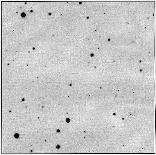
Simulated g' image for the Northern survey. The area shown is 512 x 512 pixels, and the exposure time is 55 sec.
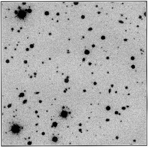
Simulated g' image for the deep Southern survey. The area is 512 x 512 pixels, and the exposure time is 1650 sec.
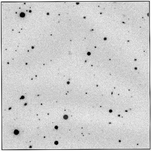
Simulated r' image for the northern survey.
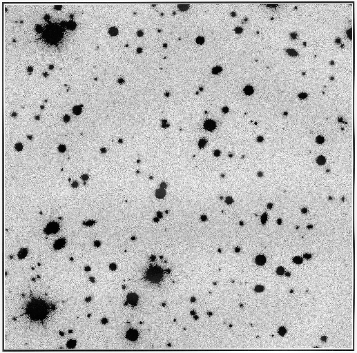
Simulated r' image for the southern survey.
We can test individual components of the data reduction software using simulated images like those described above. However, we also want to test the operation and integration of the full photometric pipeline, and for this we need a complete data stream that looks as if it is coming from the telescope. The third tier of our simulated data system turns a catalog covering a long strip of sky into such a data stream, including observation logs, astrometric and photometric parameters, postage stamps, quartiles, star lists, and raw (un-flattened) image frames (see Chapter 10, Data Systems, for details). We use realistic values for atmospheric extinction, sky brightness, atmospheric refraction, and so forth, and even include real astrometric standard stars from the standard catalogs. We prepare the test data in the actual format of the survey system, on DAT tapes.
We can use these simulated data to ask fairly detailed questions. If the sky brightness slowly increases over the duration of a photometric scan, does the photometric calibration software correct properly? What is the relative performance of the system at low and high Galactic latitudes? While the test year will no doubt bring some software surprises, the use of simulations has allowed us to have the data system integrated and largely debugged before the telescope itself is fully operational. The ability to use the same underlying data with varying degrees of complication will help isolate problems during debugging. The existence of a catalog with the "right" answers corresponding to a given simulation allows us to do regression testing in a detailed and quantitative way.
Bahcall, J., and Soneira, R. 1984, ApJSuppl 55, 67.
Coleman, G.D., Wu, C.-C., and Weedman, D.W. 1980, ApJSuppl 43, 393.
de Vaucouleurs, G., 1948, Ann. D'Astrophys. 11, 247.
Frei, Z., Guhathakurta, P., Gunn, J.E., & Tyson, J.A. 1996, AJ 111, 174.
Gould, A., Bahcall, J.N., Maoz, D., and Yanny, B. 1995, ApJ 441, 200.
Gunn, J.E., and Stryker, L.L. 1983, ApJSuppl 52, 121.
Moffat, A.J.F. 1969, AstrAp 3, 455.
Park, C. 1990, Ph.D. Thesis, Princeton University.
Postman, M., and Geller, M.J. 1984, ApJ 281, 95.
Racine, R. 1996, PASP 108, 699.
Turnrose, B.E., 1974, PASP 86, 545.
van der Kruit, P.C., and Searle, L., 1981, AstrAp 95, 105.