The Circular Polarized Alfven Wave Test |
Toth, G., "The ∇⋅B = 0 Constraint in Shock-Capturing Magnetohydrodynamics Codes", JCP, 161, 605 (2000). The test is described in section 6.3.1.
We initialize the problem described in Toth's paper; ρ = 1, P = 0.1, V⊥ = 0.1 sin(2πx||), B⊥ = 0.1 sin(2πx||), and Vz = Bz = 0.1 cos(2πx||) with γ = 5/3 and x|| = (x cosα + y sinα) where α is the angle at which the wave propagates with respect to the grid. Here V⊥ and B⊥ are the components of velocity and magnetic field perpendicular to the wavevector. They are related to the components stored on the grid Bx and By via B⊥ = Bycosα - Bxsinα, and B|| = Bxcosα + Bysinα.
For 2D the computational domain is of size Lx = 2Ly, with Nx = 2Ny (this is not as efficient as Toth's Nx x 2 grid). Thus, the grid is rectangular, but each cell is square. The wave propagates along the diagonal of the grid, at an angle θ = tan-1(0.5) ≈ 26.6 degrees with respect to the x-axis. Since the wave does not propagate along the diagonals of the grid cells, we guarantee the x- and y-fluxes are different; that is the problem is truly multi-dimensional.
We use the analytic solution for the magnetic field to compute a vector potential at cell corners, and then difference this potential to compute the initial face-centered magnetic fields.
The wave is an exact nonlinear solution to the MHD equations, allowing one to test the algorithm in the nonlinear regime. Although nonlinear amplitude Alfven waves are subject to a parametric instability which causes them to decay into magnetosonic waves (see Del Zanna, Velli, & Londrillo, A&A 367, 705, 2001), the instability should not be present for the parameters defined here. Since the problem is smooth, it can be used for convergence testing. Running the test with smaller pressure (higher β) and/or larger amplitudes is a good test of how robust is the algorithm.
Using standing waves (in which the fluid is moving at the Alfven speed in the opposite sense to the propagation of the wave) is a challenging test because it requires the two terms in the EMF cancel exactly. It is difficult to get this cancellation using schemes based on splitting
The movie below (which should have loaded and run automatically) shows the time evolution of Bz from a calculation on a 256 x 128 grid using the Roe solver and the second order algorithm. The "Stern special" color map from IDL is used, so white is the highest values, red the lowest. The movie demonstrates how the wave propagates across the grid. Note the wavefronts remain planar.
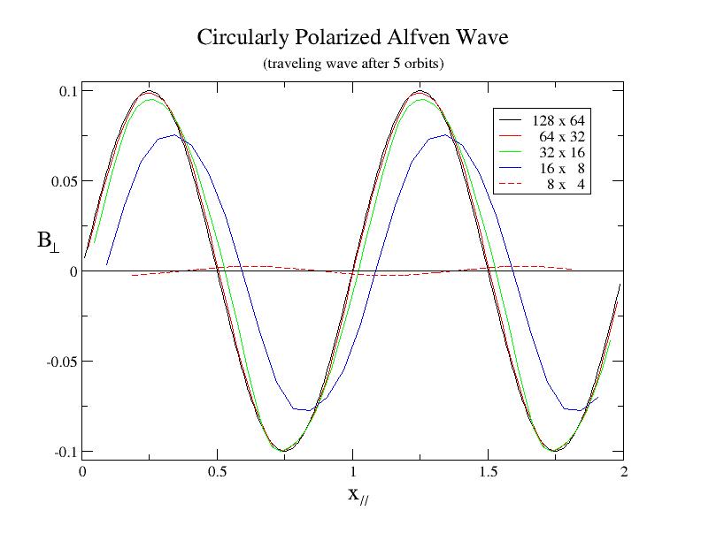
The plot below shows the transverse component of the magnetic field B⊥ after the wave has propagated 5 times around the grid at a variety of different resolutions using the second order algorithm. This plot can be compared directly to Figure 8 in Toth's paper, except the plot below shows a scatter diagram of all grid points in the calculation, rather than a 1D slice through the grid. The plot shows that along the wave front the variation is smaller than the width of the line; there is no evidence of parametric instability.
Even at the lowest resolution (with only 4 grid points per wavelength in the y-direction), the wave is evident. The amount of diffusion is less than implied by the plot, since volume-averaging strongly reduces the extrema in the initial conditions at this resolution.
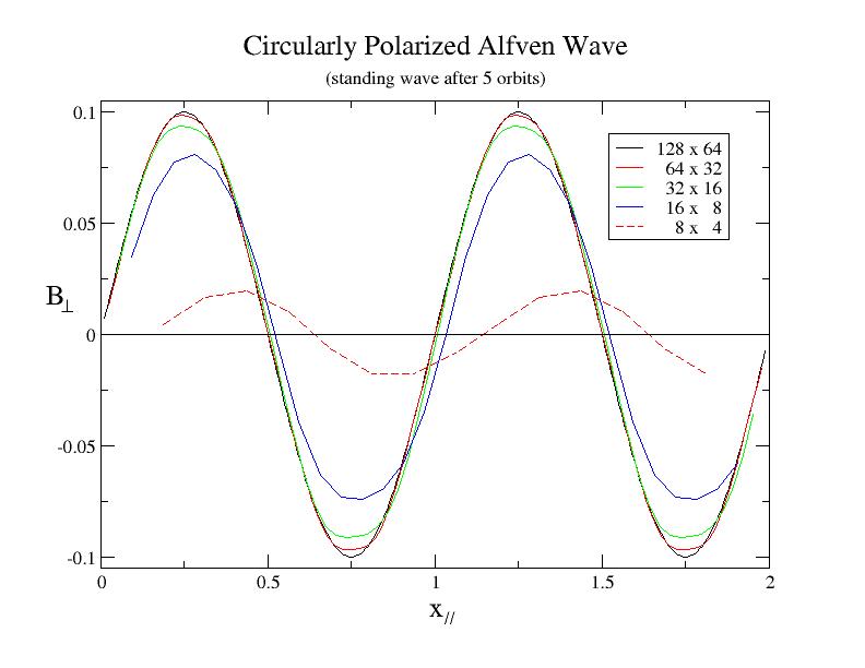
The plot below shows the transverse component of the magnetic field B⊥ at a variety of different resolutions using the second order algorithm for a standing wave after the same amount of time as shown for the traveling waves above (that is, after 5 grid crossing times at the Alfven speed). This plot can be compared directly to Figure 9 in Toth's paper, except once again the plot below shows a scatter diagram of all grid points in the calculation, rather than a 1D slice through the grid. Note the diffusion is less for standing waves at every resolution, as expected.
Now the grid is of size 2L X L X L, where L=1.5. The wavevector is taken along the grid diagonal. The background state and wave amplitude is identical to the 2D test. We use a grid with 2N X N X N grid points. The plot below shows the amplitude of the transverse component of the magnetic field for a travelling wave after 5 crossing times, computed using the HLLD solver at third-order, for N=8 (dot-dash), N=16 (dashed), N=32 (dotted), and N=64 (solid). There is excellent agreeement with the 2D results above.
The plot below shows the converge of the L1 error norm in the 3D test after one crossing time, using the HLLD solver and the CTU unsplit integration algorithm computed at 2nd (solid) and third (dashed) order. We find at least 2nd order convergence for this smooth but nonlinear wave.