

Activity
The following activity contains many graphs of supernova
brightness as a function of time (The data contained in this activity is
from BVI Light Curves
for 22 Type Ia supernovae 35. 35.
Purpose: To derive a relationship between supernovae
distances and their redshifts.
Materials:
-
Copies of directions, light curves, and spectra for each
student
-
graph paper
-
straight edge
-
calculators (optional)
Procedure (for teachers):
-
Complete an introduction with the students explaining the material
from the Supernovae
Background Section
- Have the students complete calculations and make a graph (on graph paper)
of the distance modulus versus red shift for the nine supernovae listed
below using the directions for students also found below.
- Have the students approximate or find a best fit line (a straight line!)
on their graph. This graph is known as a Hubble diagram because it shows
the relation between distances of astronomical objects and their red shift,
or in other words that the farther away an object is the faster it is traveling
away from you. It also shows that at some time in the distant past the
world was much hotter and denser. In other words, if everything that we
can see now is traveling away from us, then at some time in the past they
must have been much closer to us. This concept is known as the Big Bang.
See the activities in the Expanding
Universe Section for further explanation of this concept.
- Have the students find the slope of the best fit line. The slope is an estimation of Hubble's Constant. This constant can then be used to estimate the age
of the universe Age=1/Hubble's constant. If students
have completed the Red
Shift Lab, this is the same type of graph that is made at the end and students should compare their values from the two experiments just as astronomers do to check their own answers.
- If you wish to account for the force of gravity which
works against the cosmological expansion which is described by Hubble's
constant, the age of the universe can be calculated:
Age=2/(3*Hubble's constant).
(This is an approximation
that is only correct if the universe is flat and matter dominated. See Curvature of the Universe Background to learn more about the Shape of the Universe.)
Students should compare the graphs and estimations of
Hubble's constant that they calculated using supernova data with those
they calculated using red shift. Since astronomers have no real way of
"checking" their answers to see if they are right (for example by using
a meter stick to measure the 'actual' distance to a supernova) they must
rely on many different distance indicators and their estimation of error
in those measurements to see how close they think their estimates are.
Also students can notice the difficulties of using real data in the supernova
lab. Some of the points will not fall on a straight line, this is because
we are using a simple technique to estimate the distance to the supernovae.
When the astronomers calculated this same table they got answers that fell
much closer to a straight line because they used a more complicated technique.
You can see their graph
here
on page 29. For comparison, here is a Hubble Diagram I made using the online version of this lab.
The materials needed for the lab can be found below or here in .pdf form, including
detailed instructions I gave when teaching this lab in an advanced physics
class. The red shift which is listed in the table is really a number which
has been calculated (log (the speed of light*the red shift)) but shows
the same relation when plotted against the distance modulus. You may want
to use the red shifts listed in the table rather than having the students
calculate the red shift by hand as the precision required might be too great
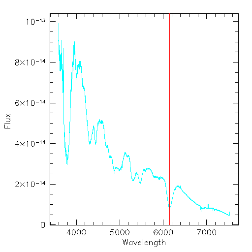
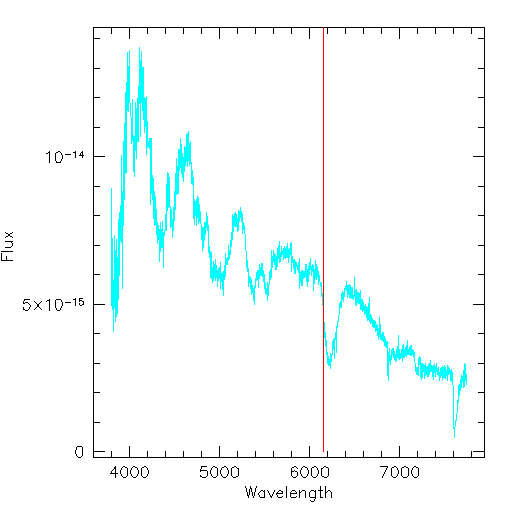
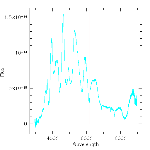
for the error which is acquired by hand measure. You can pass out some
of the spectra so that students can try to understand how the red shift
measurement is made, and then use the tabulated data for their graphs.
Alternatively, instead of printing out all of these materials
and completing the lab by hand, both the light curve measurements and the
red shift measurements can be made online in the next section. This online
activity does require some Java functions on the web browser so make sure
that your school's computing facilities can handle the program before
bringing the students to the computer lab.
Directions: Supernova Lab
-
Examine the light curves for each supernova to get a feel
for how they all look.
-
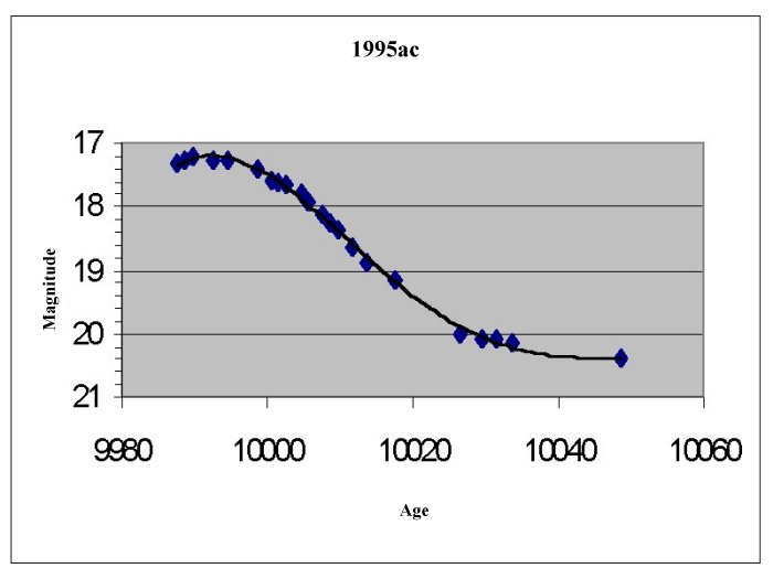
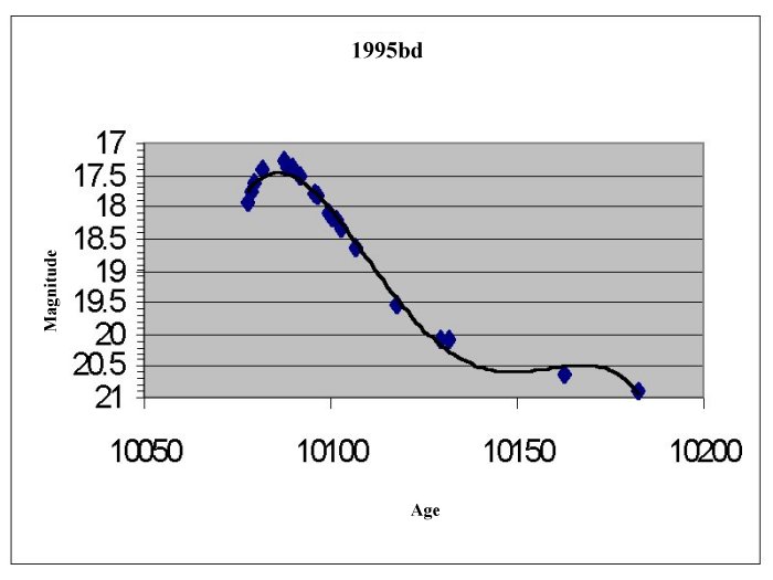
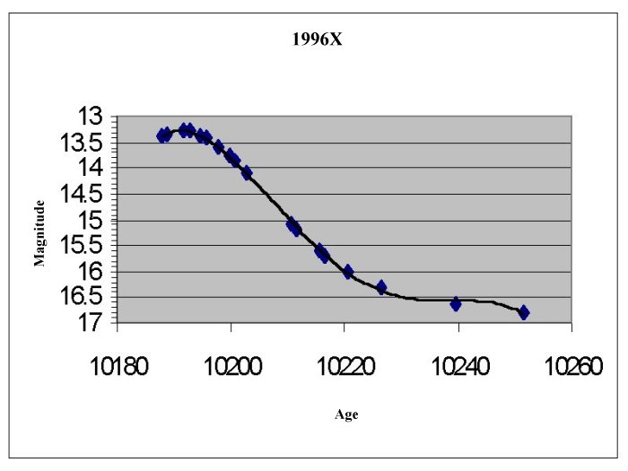
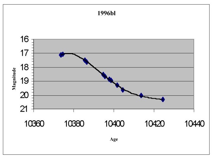
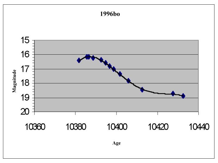
For each supernova find the maximum brightness (m) on the
curve. Remember the lower the number the brighter the supernova is.
-
Find and record the distance modulus for each supernova,
the distance modulus is defined: D=m-M, where m=the observed maximum brightness
and M is the absolute brightness for supernova -19.12.
-
Use the Distance modulus (D) to find and record the actual
distance in parsecs: d(distance in pc)=10(D+5)/5 and in km 1pc=3.09x10¹³km.
-
Make a plot of the Distance modulus versus the redshift
as listed in the table.
-
Draw a line on the graph which you think comes nearest to
the most of your data points as possible.
-
Try to find a relationship between the speed and the distance. (How does one relate to the other,
could you suggest a mathematical
equation? Remember this is real data so there may be some error and the
equation may not be exact.)
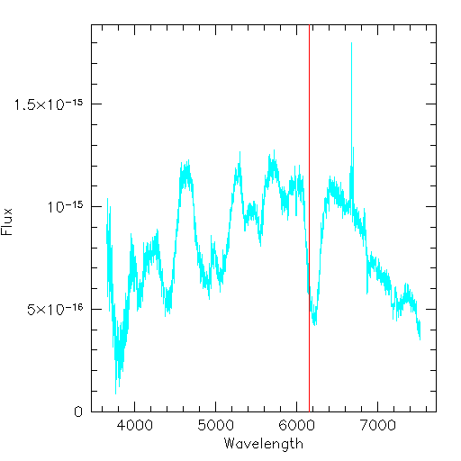
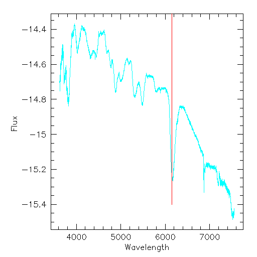
Light Curves
Supernovae Spectra
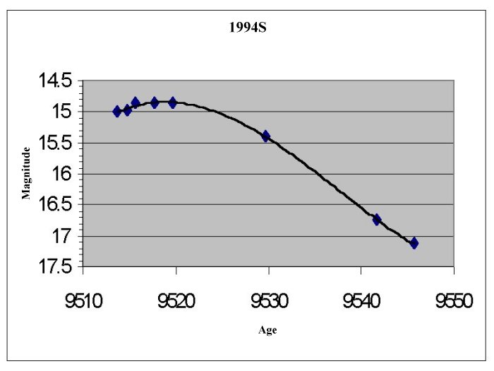
Supernova 1994S

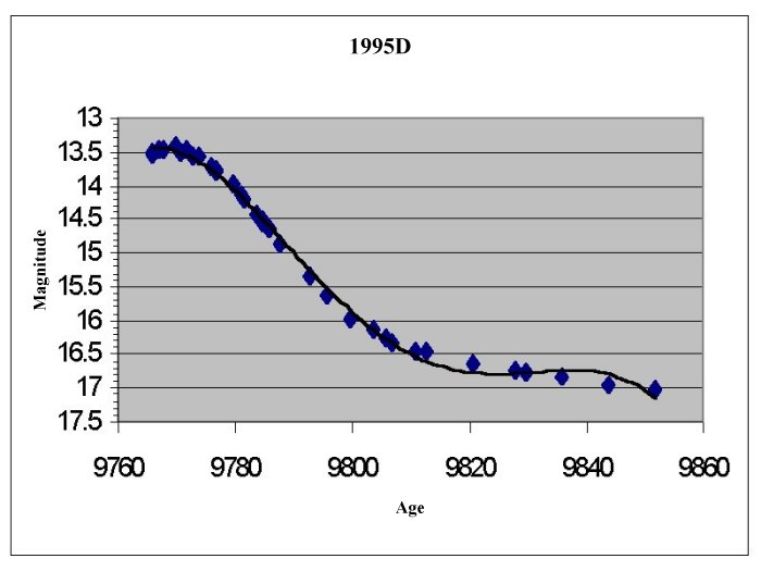
Supernova 1995D
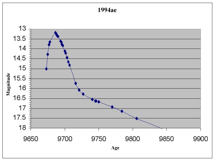
Supernova 1994ae
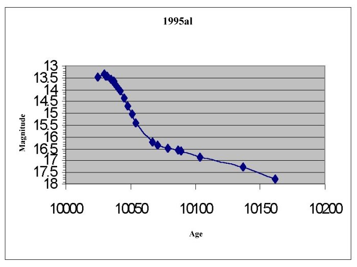
Supernova 1995al
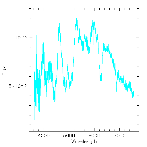
Supernova 1995ac
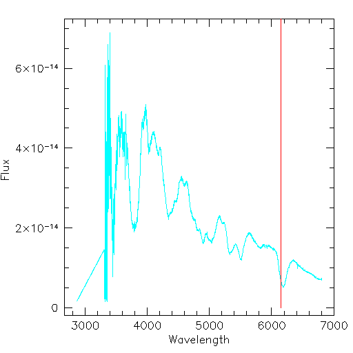
Supernova 1995bd
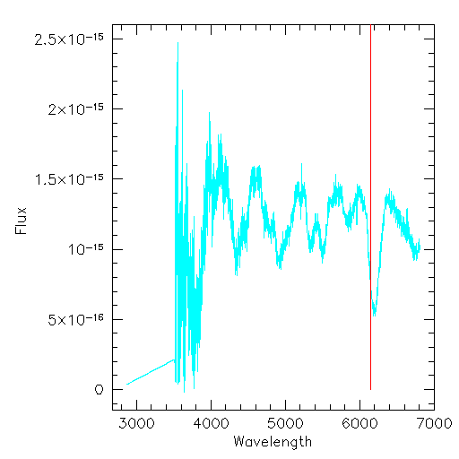
Supernova 1996X
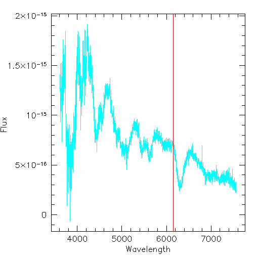
Supernova 1996bl
Supernova 1996bo
Supernovae Red shift Table
| Supernova |
|
Redshift |
| 1994S |
|
3.658 |
| 1995D |
|
3.293 |
| 1994ae |
|
3.107 |
| 1995al |
|
3.188 |
| 1995ac |
|
4.176 |
| 1995bd |
|
3.681 |
| 1996X |
|
3.308 |
| 1996bl |
|
4.033 |
| 1996bo |
|
3.714 |
Back
| Next
|