Linear Waves Test |
Sturrock, P.A., Plasma Physics, CUP, Chpt. 14; Shu, F., The Physics of Astrophysics, Volume II Gas Dynamics, Univ. Sci. Books, Chpt. 22.
The density, velocity, magnetic field, and total energy are all set to constant values initially. These values can be chosen so that the wave speeds are all well separated, and so that (in MHD) the wavevector is at an arbitrary angle to B. The precise values chosen for the tests described here are given in the appropriate results section below.
The wave is added to as a perturbation to these constant values of the form δ U = A R sin (2 π x). Here U is the vector of conserved variables, A is an amplitude, and R is the right-eigenvector corresponding to the desired wave family. To aid others in comparing to our results, we give the components of R for each test in the appropriate results section below. For all the tests shown here, A = 10-6. For 2D and 3D problems, the face-centered components of the magnetic field are initialized from a vector potential located at zone corners.
The length of the computational domain is set to be one wavelength. Periodic boundary conditions are used. After the wave has propagated one wavelength, we measure the error in the numerical solution by computing the norm of the vector resulting from summing the absolute value of errors in each variable over the grid, that is we compute ε = || Δ U || = [&sumk (&Delta Uk)2]1/2, where Δ Uk = ∑i |Uk,in - Uk,i0| / Nx. Here, Uk,in is the numerical solution for the k-th component of the vector of conserved quantities at grid point i and time level n, Uk,i0 is the initial numerical solution (at time zero), and Nx is the number of grid points. Note the initial solution Uk,i0 is just the analytic solution which has been discretized to the grid using volume averaging. Since the discretization of the initial condition also introduces error, to measure the error in the integration algorithm it is important to compute errors relative to the initial condition Uk,i0 rather than the analytic solution. In 2D (3D), summation over j (k) is required as well.
To compare to the results given here, it is important to (1) use the same amplitude for the wave, (2) compute the errors in exactly the same way, and (3) compute the errors at exactly the same time.
This is an excellent quantitative test of the accuracy and convergence rate of a numerical algorithm. The only drawback is that it involves only linear amplitude oscillations. Thus, this test is not characteristic of the kind of problem codes are written to solve in the first place (after all, the dynamics of linear waves can be treated analytically). A code which does well on this test may still be very poor at shock-capturing. Still, it is nice to know an algorithm reduces to the correct answer in the linear regime. Moreover, since virtually all schemes are first-order for discontinuities such as shocks, smooth problems like this are the only way to measure the actual convergence rate of higher-order schemes.
The test is sensitive to both diffusion error (the rate at which the amplitude of the wave decreases), and dispersion error (the difference between the speed at which the wave propagates in the numerical versus the analytic solution). The error norm plotted here contains contributions from both. However, one could plot the error as a function of position or phase to track each individually.
Finally, this test has proved very useful at detecting coding bugs. The errors for left- and right-going waves of the same family should be identical, for example. Also, if the errors do not converge, something is wrong somewhere. We found it necessary to use double precision and very small wave amplitudes to eliminate round-off error and nonlinear effects.
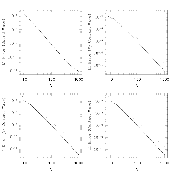
In this case, we set ρ = 1 and P = 1/γ, with γ = 5/3. If the components of U are ordered U = [ρ, ρVx, ρVy, ρVz, E], then the right-eigenvector for a left-going sound wave is R = [1,-1,1,1,1.5]. The absolute error in propagating a sound wave to the left one wavelength computed with Athena using the HLLC solver and both second order (dashed line) and third order (solid line) methods as a function of the number of grid points Nx is given below. We also given the error in an entropy wave, in which case we set Vx = 1.0 everywhere.

Note the third-order scheme gives lower errors, and slightly faster than second-order convergence (even though formally it is a second-order scheme).
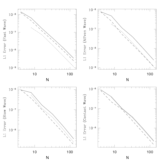
In this case, we set ρ = 1, P = 1/γ, bx = 1, by = √ 2, bz = 0.5 (where b = B / (4π)1/2) with γ = 5/3. Thus, the fast magnetosonic speed is 2.0, the Alfven speed is 1.0, and the slow magnetosonic speed is 0.5. Tables of the right-eigenvectors for left-going waves can be found here. The absolute error in propagating each of these waves to the left one wavelength computed with Athena using the Roe solver (solid line), HLLD solver (dashed line), and HLLE solver (dotted line) at third-order as a function of the number of grid points Nx is given below.
The errors in the HLLD and Roe solvers are nearly identical. Both are significantly better than the HLLE for all but the fast wave, as expected. The HLLE solver converges at exactly second order, the others slightly faster.
In this case, we use the same values as for the 1D adiabatic MHD test, but we use a 2D grid of size 0 ≤ x ≤ 2 and 0 ≤ y ≤ 1. We use twice as many grid points in the x-direction at every resolution (e.g. our highest resolution is 512 X 256), thus the grid is rectangular, but each cell is square. The wave propagates along the diagonal of the grid, at an angle θ = tan-1(0.5) ≈ 26.6 degrees with respect to the x-axis. Since the wave does not propagate along the diagonals of the grid cells, we guarantee the x- and y-fluxes are different; that is the problem is truly multi-dimensional.
The error (now scaled to the initial wave amplitude) in propagating each of these waves to the left one wavelength computed with Athena using the Roe solver and third order reconstruction as a function of the number of grid points in the y-direction (which has the fewest grid points per wavelength) is shown in the plot below using points marked by an 'X'. Points marked by a square are from the one-dimensional test using third order reconstruction (identical to the results given above).
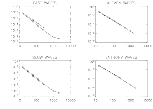
Note the amplitude and convergence rate of the two-dimensional errors is remarkable similar to the one-dimensional algorithm, despite the complexity of integrating the EMFs to cell corners, and the transformation between face-centered and cell-centered magnetic fields, which is required in multi-dimensions.
Now we use a 3D grid of size 0 ≤ x ≤ 3 and 0 ≤ y ≤ 1.5, and 0 ≤ z ≤ 1.5. The grid is of size 2N X N X N. The wave propogates along the grid diagonal, again guaranteeing a truly multidimensional test. The background state is identical to the 1D test values.
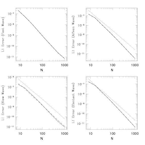
The absolute error in propagating each of these waves to the left one wavelength computed with Athena using the HLLD solver and the CTU unsplit integration algorithm at second order (solid line), third-order (dashed line) are shown along with the errors in the 1D test at second-order (dotted line). For all but the fast waves, the 3D errors are as good or better than the 1D case.
