
Kelvin-Helmholtz Instability Test |
"Hydrodynamic and Hydromagnetic Stability", by S. Chandrasekhar. Sections 101 considers the stability of a slip surfce between two fluids of different densities, section 106 considers the effect of a magnetic field on the problem. See also Frank et al., "The Magnetohydrodynamic Kelvin-Helmholtz Instability: A Two-dimensional Numerical Study", ApJ 460, 777 (1996)
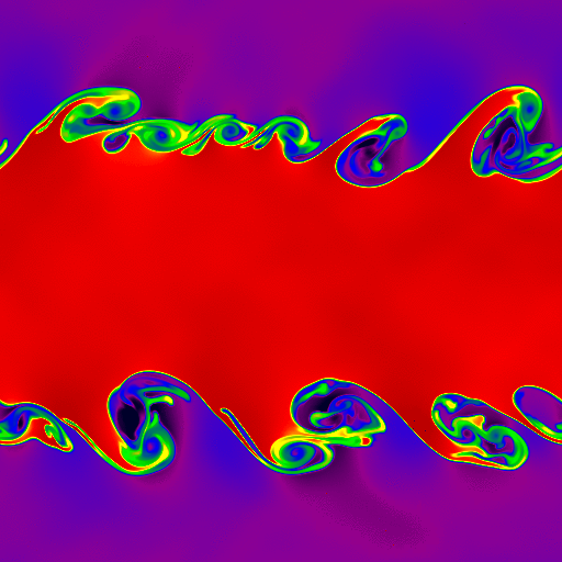
We use a square domain, -0.5 ≤ x ≤ 0.5; -0.5 ≤ y ≤ 0.5. The boundary conditions are periodic everywhere. For |y| > 0.25, we set Vx = -0.5 and ρ = 1, for |y| ≤ 0.25, Vx = 0.5 and ρ = 2. The pressure is 2.5 everywhere, and γ = 1.4, giving a Mach number of about 0.377 in the ρ = 2 gas, and about 0.267 in the ρ = 1 gas. The interface between the two oppositely directed streams is a discontinuity, that is a "slip surface". We use different densities in the two fluids to make visualization of the interface easier.
For the MHD problem, the initial magnetic field is uniform everywhere with Bx / (4π)1/2 = 0.5.
To seed the instability, we add random numbers to both the x- and y-components of the velocity with peak-to-peak amplitude of 0.01.
At early times, one can check that the growth rate of the transverse component of the velocity agrees with the prediction from linear theory. This requires initializing a single-mode perturbation rather than a spectrum of perturbations as we have done here.
At late times, once the instability has gone fully nonlinear, it is difficult to make quantitative comparisons. However, the sharpness of the boundary between the two streams is an indication of the numerical diffusion of the scheme. For example, if the HLLE Riemann solver is used, diffusion at the interface is significant enough to suppress the instability.
Results computed with Athena using the HLLC solver and the third order algorithm on a 512x512 grid are shown below at time=1.0 (on the left), and time=5.0 (on the right). The images show the density on a linear color map between 0.9 and 2.1.
Click on the right image to download a .gif movie (65MB).
|
|
|
For more quantitative comparisons between schemes, we plot the time evolution of the kinetic energy in the transverse component of the velocity (0.5ρVy2) averaged over the computational domain for a 128x128 grid (dashed line), a 256x256 grid (dot-dash line), and a 512x512 grid (solid line).

|
For the MHD problem, the initial magnetic field is uniform everywhere with Bx / (4π)1/2 = 0.5. Results computed with Athena using the Roe solver and the third order algorithm on a 512x512 grid are shown below at time=1.0 (on the left), and time=5.0 (on the right). The images show the density on a linear color map between 0.9 and 2.1.
Click on the right image to download a .gif movie (39.5MB).

|

|
For more quantitative comparisons between schemes, we plot the time evolution of the total magnetic energy, minus the initial value [(B2 - B20)/8 π] averaged over the computational domain for a 128x128 grid (dashed line), a 256x256 grid (dot-dash line), and a 512x512 grid (solid line).

|