Gravitational Potential Identification of Cores
GRID-core is a core-finding method using the contours of the local gravitational potential
to identify core boundaries, as described in Gong & Ostriker (2011). There it is shown that the
GRID-core method applied to 2D surface density and 3D volume density are in good agreement,
for bound cores.
We have implemented a version of the GRID-core algorithm in IDL, suitable for core-finding in
observed maps. The required input is a two-dimensional FITS file containing a map of the column
density in a region of a cloud.
The user's guide is available in PDF format.
The IDL source code and test files are available for download. Please cite the original paper
( Gong & Ostriker 2011) if you use the code for presentation or publication.
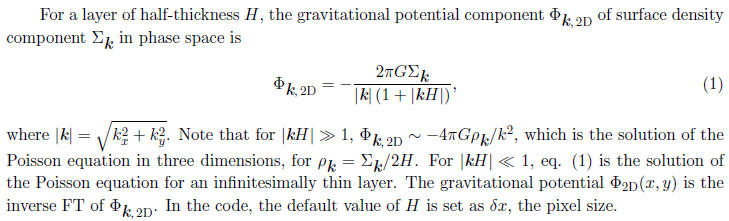
2. Gravitational potential of surface density
5. Structure of the IDL progam
GRID-core (Gravitational
potential Identification of cores) is a core-finding method using the
contours of the local gravitational potential to identify core boundaries, as
described in Gong &
Ostriker (2011). There it is shown that the GRID-core method applied to 2D
surface density and 3D
volume density are in good agreement, for bound cores. This user guide describes
how to implement
this method on observed surface density. We describe the algorithms used to find
the largest closed
contour that defines the outer core limit, and to identify the gravitationally
bound interior part of
the core. In addition, we describe use of the IDL code to implement GRID
core-finding on FITS
maps.
2. Gravitational potential of surface density
To identify cores via the
gravitational potential, we first find and mark all the local minima
of the gravitational potential; second, we find the largest closed potential
contour surrounding
each individual minimum. In the second step, we increase the contour level from
the bottom of a
given potential well step by step until it violates another minimum's marked
territory by enclosing
more than one extremum of the potential. We demonstrate this procedure in Figure
1 using a
one dimensional positive potential, -Φ . In the first step, local maxima (minima
in Φ) are marked
in a descending order; note that only pixels at extrema are marked in this step.
For the second
step, we take the local maximum "1" as an example. Starting at | Φmin|,
we decrease the isopotential
contour
level by amount of ΔΦ from the top of "1", and find the region which is
connected to "1" for
each
contour level. The blue lines in Figure 1 show the contour levels, and the
dotted blue lines show
the
identified connected regions to the maximum "1". At the 7th contour level, the
connected region
violates the territories of other maxima, because more than one extremum is
contained within the
contour (i.e. lying above the lowest blue line, in Fig.1) . The largest closed
contour of "1" is
thus defined by the 6th contour level, marked
by the red lines. We repeat this procedure on all the
local maxima and mark the
largest closed contour of each maximum.
The contour interval ΔΦ has a negligible effect on the
results as long as it is small enough. We
define the region enclosed by the largest closed contour as a GRID-core. If the
distance between
two potential minima is smaller than a certain value of pixels (corresponding to
a physical distance
which is set by the resolution), the regions associated with these two minima
are merged and treated
as a single GRID-core.
Fig. 1. Schematic of GRID-core identification method.
Gas with sufficient thermal
(and kinetic) energy will not be permanently (or even temporarily)
bound to a given core, so the gravitational potential is not the final word. The
lower density outer
parts of a core are the least bound, and most subject to mass loss.
In order to identify
only the bound regions of cores as marked by the gravitational potential,
we add thermal energy to the gravitational energy, and only assign a given
fluid element to a
core if Eth+Eg < 0. For any fluid element, the specific thermal energy is taken
to be Eth = (3/2)cs2,
for cs the isothermal sound speed, and the specific gravitational potential
energy is taken to be
Eg =Φmin - Φmax, where Φmax is the potential of the largest closed contour that
defines the core. In
the example of section 2, Φmax would be equal to the potential of the sixth
contour, i.e. -Φ max =
- Φmin - 6Δ Phi. Including a thermal energy condition decreases the area so that
(instantaneously)
bound cores are smaller than cores defined by the potential alone. The resulting
region is defined
as a bound GRID-core.
Of course, the thermal
energy can in fact be radiated away, so that gas that is initially near
the largest closed contour may become more strongly bound after the interior of
a core collapses.
Thus, the gas within the outer (unbound) GRID-core region could evolve to become
a bound core
eventually.
Since bound cores must
have Φmax −Φmin < (3/2)cs2, a value ΔΦ
~ 0.1cs2 is typically suitable
for the potential contour spacing in identifying core boundaries. This is the
default value adopted
in the code.
We define a background
surface density as the mean of the bottom 10% of the surface density;
this mean value can be subtracted from the surface density in the core region
when calculating core
masses.
5. Structure of the IDL progam
The code contains two
subroutines: "destroy_bad" and "boundcore2d." The subroutine "destroy_bad"
eliminates unresolved cores (total pixel number smaller than π r_pix_lim2). The
subroutine
"boundcore2d" calculates core properties such as the coordinates of core center, total
mass of the region
inside the largest closed contour, mass of the bound core region, the depth of
the gravitational
potential well ( Φmax −Φmin), and the total number of pixel numbers in marked
cores, and bound
regions. All the other procedures such as calculating the gravitational
potential, and core-finding
are handled in the main function. This section explains each block
in the main function.
The first block is to calculate the gravitational
potential of surface density. The surface density
in g cm−2 is obtained by multiplying input H column density by 1.42mp. To create
a periodic input
for the FFT function, we zero-pad the surface density map in a domain four times
as large, putting
the physical surface density in the lower left quarter and zeros in the other three
quarters. The next step is
to apply a forward FFT to the extended surface density map. After multiplying by
the coefficients
as in equation (1), we apply a backward FFT to obtain
the gravitational potential
of the extended
surface map. At the end of this block, the bottom left part of the gravitational
potential field is
extracted for later core-finding. Notice that the potential field is converted
to positive values.
The second block is to merge local maxima
(originally these are minima, since we use −Φ
instead of Φ) if they are too close to each other (rdistance < cls_dis).
The third block is to do GRID core-finding. The
algorithm is described in Section 3. The
block to eliminate unresolved cores is right after this block.
The calling sequence is:
output=grid core(filename, pix_size,T,cls_dist=cls_dist,dp=dp,h=h,r_pix lim=r_pix_lim)
ARGUMENTS:
filename : the name of the FITS file containing column density, where the maps is assumed to
represent NH of H nuclei (not H2), in units of cm-2
pix_size : the pixel resolution of the input column density map, in units of pc
KEYWORDS:
T : temperature of the cloud (assumed isothermal), in units of K; the default value is 10 K.
dp : the interval between potential contour levels, in units of cs2 = kT /µ; the default value is 0.1.
cls_dist : the closest distance between two local potential minima, in units of pix size; the default value is 6.
h : the minimum thickness of the 2D layer, in units of pix_size; the default value is 1.
r_pix_lim : the minimum radius for a core to be considered resolved, in units of pix size; the default value is 3,
half of cls_dist.
OUTPUTS:
1. Two FITS files containing the marked regions identifying cores, e.g.: lcc_0.100.fits (GRID- cores),
lcc_b_0.100.fits (bound GRID-cores). The suffix gives the value of dp (“0.100” for the default).
2. A FITS file containing a map of the computed gravitational potential phi.fits ( in units of [km/s]2).
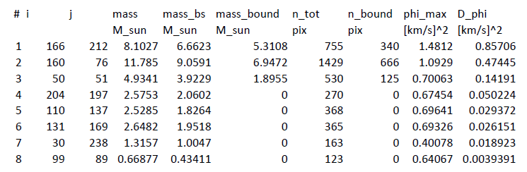
3. A data file containing the properties of each core: location of potential minimum, total mass of marked region,
background-subtracted mass of bound region, pixel numbers of both total and bound regions, gravitational
potential |Φmin| at the core center, gravitational potential depth Φmax −Φmin.
4. A postscript file showing the marked regions identifying cores: core_on_surfd_0.100.ps .
Examples of how to run the code:
1. Setting all keywords –
.run grid_core
output=grid_core(“column.fits”,0.011,10.,cls dist=6,dp=0.01,h=1.0,r pix_lim=3)
2.Using default keywords –
.run grid_core
output=grid_core(“column.fits”,0.011,10.)
For a column density map (figure 2, 256x256), the potential map is shown in Fig. 3, and the marked GRID-core
and bound GRID-core areas are shown in Fig. 4 and Fig. 5 respectively. Fig. 6 shows the marked GRID-cores
and bound GRID-cores on the column density map.
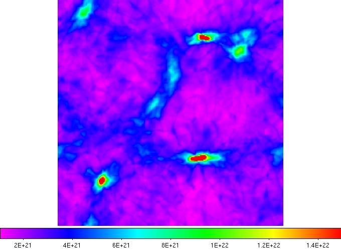
Fig. 2 Column density map. Color scale represents the column density (logNH).

Fig. 3 Potential map of the above column density map. Green curves show the contours.
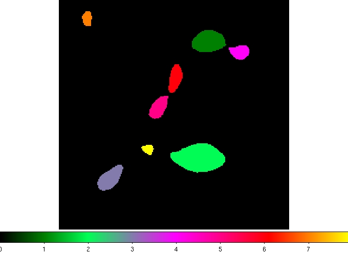
Fig. 4 Identified GRID-cores. Colors represent different core indices.

Fig. 5 Identified bound GRID-cores.
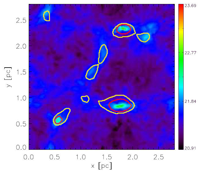
Fig. 6 Identified GRID-cores (yellow curves) and bound GRID-cores (red curves) superposed on the
column density.
The parameters of identified cores are list below: